Exploring the methodology of NFT price definition
Original title: "Exploring NFT Price Distribution Across Collections"
Original author: Gringotts DAO
Original compilation: Block unicorn
< br>
NFT categories such as virtual lands, PFPs (NFT portraits) and game assets are common frameworks for valuing items and collectibles. However, a less-discussed and sometimes counterintuitive property of these assets is their price "rank" in the collection, and how assets of the same price class behave in collections and NFT classes.
Gringotts DAO's mission is to be a one-stop shop for NFT holders to access liquidity. With the rapid emergence of new NFT financialization protocols, we set out to evaluate the effect of different approaches in the context of users seeking liquidity for NFT types. Instead of focusing solely on asset classes, we looked at a property that all of these assets share—their prices.
More specifically, we tried to answer 3 questions:
NFT in the entire market What is the distribution of prices?
Are price distribution patterns emerging, and if so, how common are they?
From these distributions, how do we define price "tiers" that might make a given NFT more suitable for some liquidity methods than others?
One of the main findings is that items in collections and NFT categories may behave more similarly than items in the same collection. Therefore, price distribution analysis can give users and developers a more comprehensive understanding of where liquidity is best found, and the potential market for financialization methods.
Methodology
NFTBank is an algorithmic asset valuation product that uses machine learning based on Past pricing of similar assets to predict NFT prices. We extracted more than 3 months of data from NFT Bank. The first is December 15, 2021 (279 collections, about 2.4 million NFTs, about 3.7 million ETH market value), and then January 13, 2022 (540 collections, about 14.2 million NFTs, about 8.9 million ETH market value), Most recently on February 27, 2022 (538 collections, about 14.8 million NFT, about 6.5 million ETH market cap)
This article explores in depth 4 observations we found:
1. The price distribution is usually very concentrated between and within sets.
2. There are 5 main "shapes" of price distributions that don't seem to be related to NFT "categories" (PFP, games, virtual land, etc.).
3. The price distribution generally remains unchanged. For 75% of collectibles, the price distribution remains constant across time points. For those that change, it is toward a "relevant" shape.
4. For collections with exponential decay and lognormal-like distribution (60% of collections), we can define and examine bottom, middle and top assets the behavior of.
Concentrated price distribution
Among each series, the market is concentrated in the top 10 series More than 60% of the market capitalization, the (normalized) Gini coefficient is about 0.9.
Among collectibles, most price distributions follow a pattern where most items are priced close to the reserve price. The few remaining items make up the majority of the price range and thus contribute significantly to the market value of the collection.
Example of normalized price distribution chart:
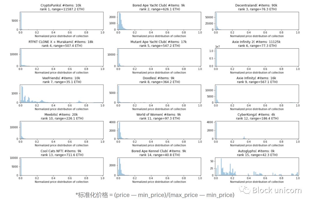
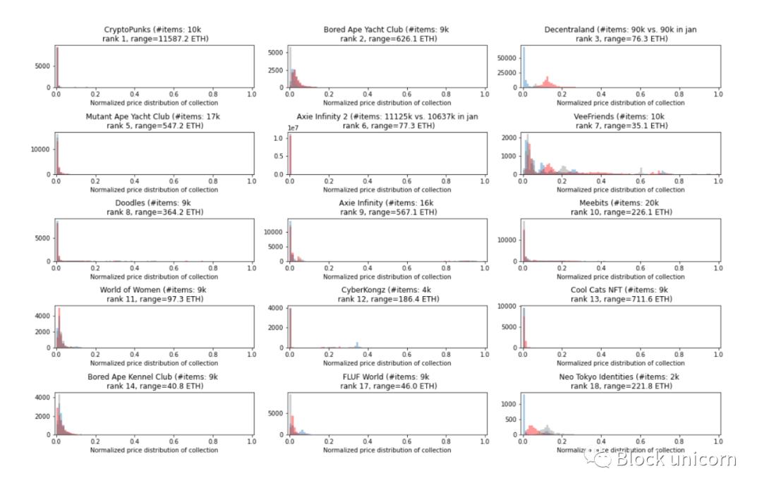
In these charts, The x-axis is divided into 100 equal parts, so for example the first chart (CryptoPunks) shows that almost all punks are priced in the top 2% of the full price range.
This is promising for NFT financialization products that are most suitable for on-site projects, for example, liquidity pools like NFTX can act as "on-site AMM", which provides instant liquidity for NFT owners, who can trade assets on the market with the pool.
Collections with a large number of on-market items and reliable price feeds (those that are frequently traded across many different unique addresses) can also serve as a P2Pool lending product collateral. This is because floor assets can often be treated "the same" and thus do not require manual valuation. Loan terms can be automated once price feeds and automated means of assessing risk are plugged in.
However, in the example above, note that some collections (such as VeeFriends and Decentraland) do not fit into this "model is floor price" model. In fact, the price distribution pattern falls into one of 5 different shapes, which brings us to our next observation.
There are five main forms of price distribution
In each In the series, the shape of the price distribution we observed was:
1) Exponential Decay. These are collectibles where most of its merchandise is priced on the floor, and there's a long tail of high-ticket items. About 40% of the collections we sampled exhibit this profile. Examples include Cryptopunks, RTFKT Clone X + Murakami and Mutant Ape Yacht Club

2) The quasi-lognormal distribution has a similar shape to an exponential, but the pattern is slightly above the floor. About 20% of the collections we sampled exhibit this profile. Examples include Bored Ape Yacht Club, Sandbox LAND, and Decentraland.
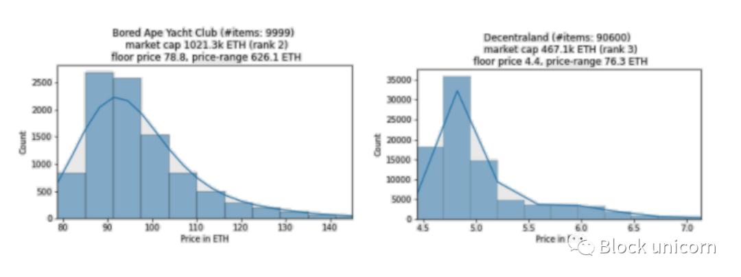
3) Symmetrical (or similar to normal) distribution means that the assets are highly concentrated around the average price and gradually decrease on both sides. About 5% of the collections we sampled exhibit this profile. Examples include Anonymice, Blitmap, and Rollbots.
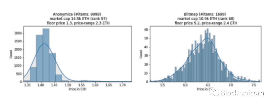
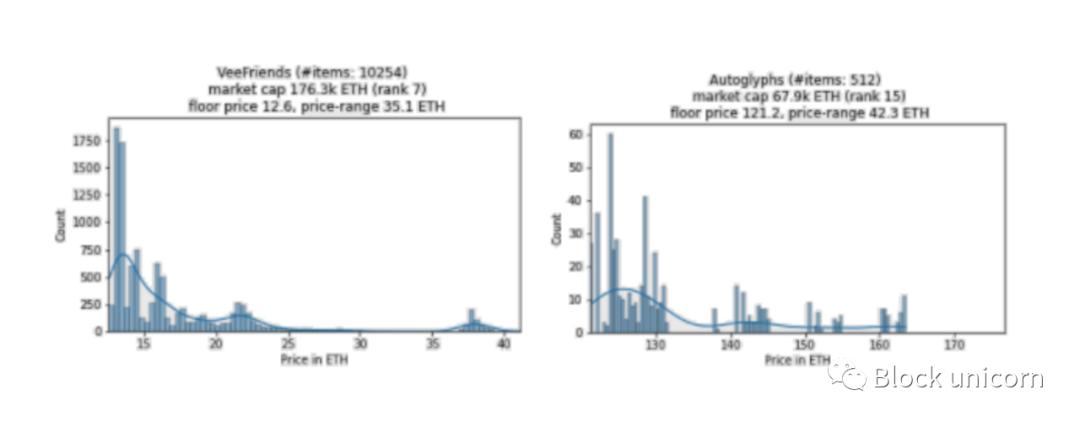
4) Multimodal distribution exhibiting multiple bumps and spikes over a wider range. About 20% of the collections we sampled exhibit this profile. Examples include VeeFriends, Autoglyphs, and FLUF World.
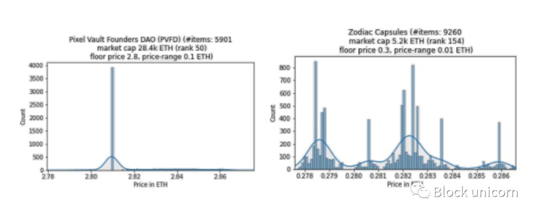
5) The point distribution pattern has one of the above shapes, but the price is distributed at <0.1 ETH. Since we define this as roughly the same price, we label these as "point distributions". This shape is a common feature of the smaller hat collections (except for PVFD, none of the top 100 collections have this shape) - so they act as filters. About 15% of the collections we sampled exhibit this profile. Examples include PVFD, Zodiac Capsules or PEGZ.
Interestingly, the NFT category (PFP, virtual land, game assets, etc.) is independent of the shape of the price distribution. For example, the virtual land NFTs in Cryptovoxels, Decentraland, and Somnium Space all have different distributions (exponential, lognormal (symmetric in Jan/Dec data, respectively), and multimodal).
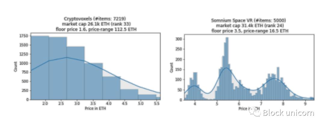
The price distribution is likely a function of inherent characteristics of the collection itself, rather than the NFT category it belongs to. For land, this could be location, plot size, foot traffic (income generating potential), land that is already built and therefore sold at a premium, etc.
Next, we investigated whether these price distributions changed over time.
The price distribution (usually) remains the same
Due to limited data here (3 data points), only time will tell if the analysis here will continue into the future. Looking at the normalized prices again, we can see that the price distributions for December (gray) and January (red) usually (but not always) coincide with or at least have a similar shape to that for February (blue).
Of the 537 collections included in both January and February data, 166 had a change in price distribution shape (30%). We also saw a similar proportional change (25%) from January to December. That might sound like a lot, but keep in mind that the categorization of the distribution shape of the set above is a bit vague, since we're not too strict about the cutoff.
For example, one can distinguish between exponential decay and lognormal: "if mode > bottom price => lognormal". Looking at the mode-to-floor ratios below, we chose a more relaxed definition and allowed modes to be even 10%-20% above the floor because we looked at the fitted distribution to classify their shape.
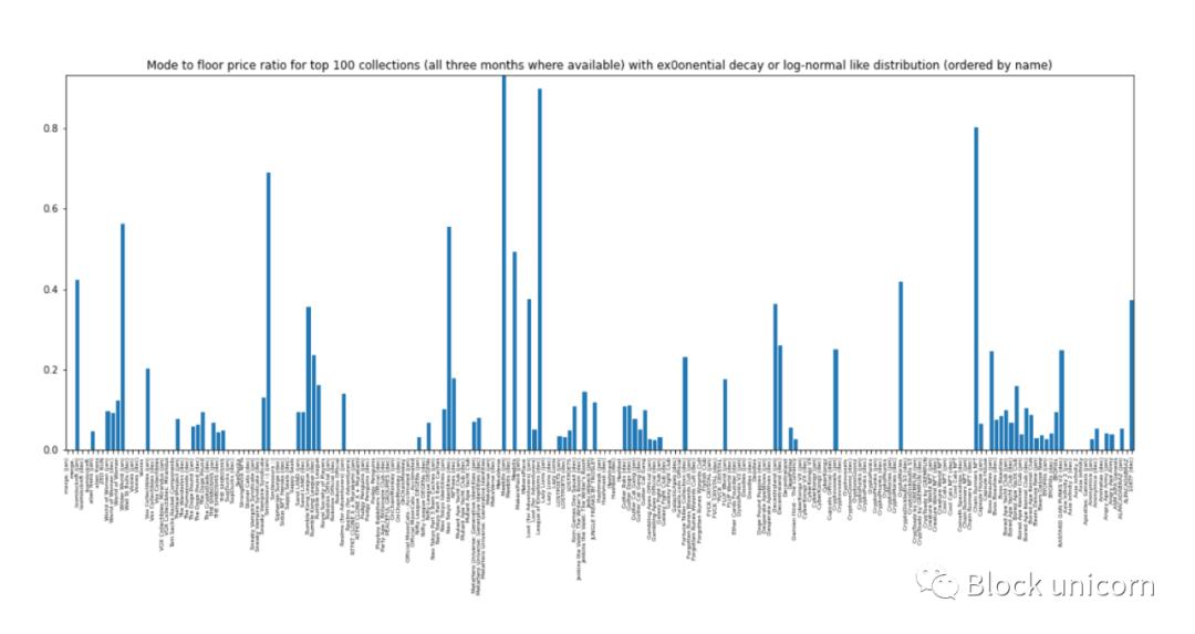
On this basis, we consider the exponentially decaying distribution and the lognormal distribution to be "related".
For the observed change in price distribution:
~42% change to and from point distribution. Point distributions come in one of the other four forms, but with very narrow price ranges.
~26% from exponential decay or lognormal to multimodal. The definition of this class is also softer, since our distribution usually only has one schema. We define this shape to separate distributions like VeeFriends and its several bumps (modes) from other shapes.
~22% is the exponential decay to/from the lognormal distribution (this number would be much higher if we took the strict approach ).
The remaining variation of ~10% is symmetrical, with the lognormal accounting for the majority (6%). This is also due to the fact that the line between the lognormal and symmetric distributions is rather loosely defined (i.e. the two shapes are also "correlated").
Define the price ladder
Based on the above observations, we look for A collection of dynamic shapes is used to define the price ladder, as floor prices can serve as reasonable anchors here. Of course, since an "absolute" floor may simply be the lowest-priced item, we would like to find an appropriate multiplier to classify more items as the floor.
Defining the lower bound: We studied different lower bound quantiles and their ratios to the floor price.
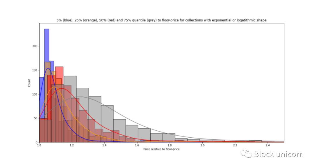
Of the 800 items in the collection, about 90% have a median price below 1.4*reserve. Choosing a threshold here depends more on the use case we have in mind: if we include a larger share of collection items further to the right, we run the cost of expanding their price range, making the collection less homogeneous .
To get the threshold to work for about 90% of the collection, the threshold is:
1.3 gives out of the 25% quantile (thus covering 25% of the items).
1.4 gives about 50% quantile/median.
1.75 represents the ~75% quantile.
A collection of less than 30% may be too small, and a price range of [reserve price, reserve price*1.75] may be too wide. Therefore, we choose a multiplier of 1.4 as the lower bound. In other words, "floor" items are items within the price range of [floor price, floor price *1.4]. For two-thirds of the collections, this includes 75% of the items.
Defining top-level items: We can follow a similar route using top-level quantiles:
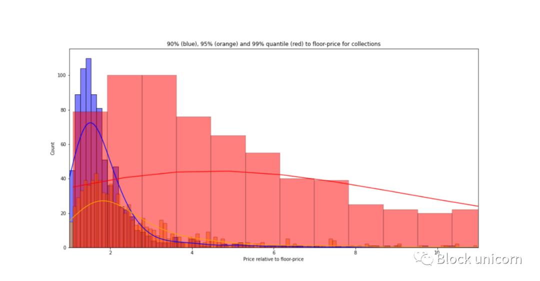
2.5 threshold covered 90% of favorites - 85% of those 800 favorites. It also includes 95% of collections in two-thirds of collections, and even 99% of collections in ~20% of collections. In other words, a threshold of 2.5 would place the top 10% of assets in the "top" bucket of 90% of the set.
Again, we can do more exclusive operations on the set, for example increasing this threshold to 4.
Under these definitions of bottom price and top price, we can define mid-range products with prices between [bottom price*1.4, bottom price*2.5] as . Now let's look at the features of these price ladders.
Define the characteristics of the price tier
Items priced at reserve price to reserve price* 1.4.
Floors typically make up 50-75% of a collectible and 25-50% of its market value. Their volume and homogeneous behavior make them suitable for liquidity pools, effectively acting as "floor AMMs", where users can earn benefits on the trading activities of assets on the floor and enjoy the deepest liquidity compared to other price tiers.
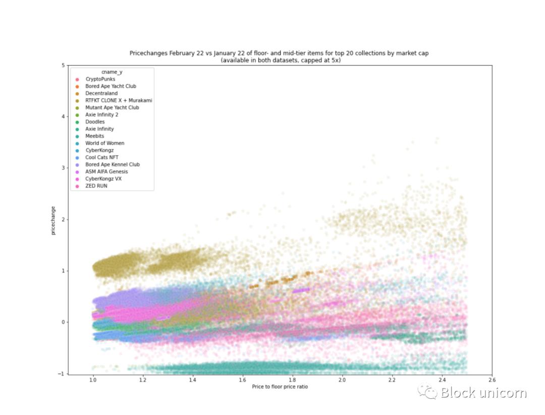
Project price base price*1.4 to reserve price*2.5.
The floor price usually accounts for 20%-40% of the product and 10%-20% of the market value of the collection. As things stand, mid-range products are probably the least profitable to trade, as they require less liquidity than pit trades, and they have less exposure to reflexive upside than Grails. Aggregates, where the modes are mid-range (those with symmetric price distributions), are likely to be the ones in which many users are more interested in the properties or utility of the asset itself than the price. For example, a virtual land floor may be too small or in an unprofitable location, while a large, high-traffic land may be too expensive or not for sale. Therefore, land buyers look for assets with good location, lot size and price
If it turns out that the floor price contains some "temporary" items, that is, the floor price increases or price falls, then this could be a layer of speculation and related hedging applications.
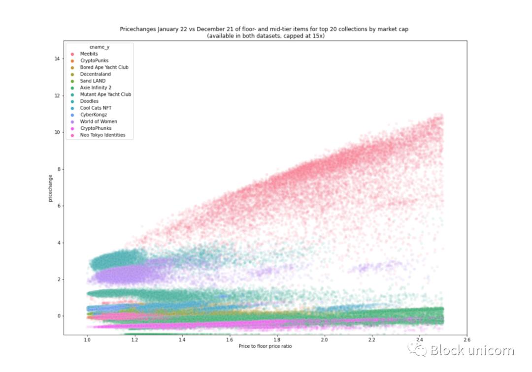
TOP or top item, commodity pricing>base price*2.5.
The head item usually accounts for 5%-10% of the merchandise and 20%-40% of the market value of the collection. Antique sales are very noisy and have high price fluctuations, behaving like "traditional" art or high-end items in real estate. Although their transaction volume and speed are low, they have good potential to be used as collateral or for liquidity through spinoffs.
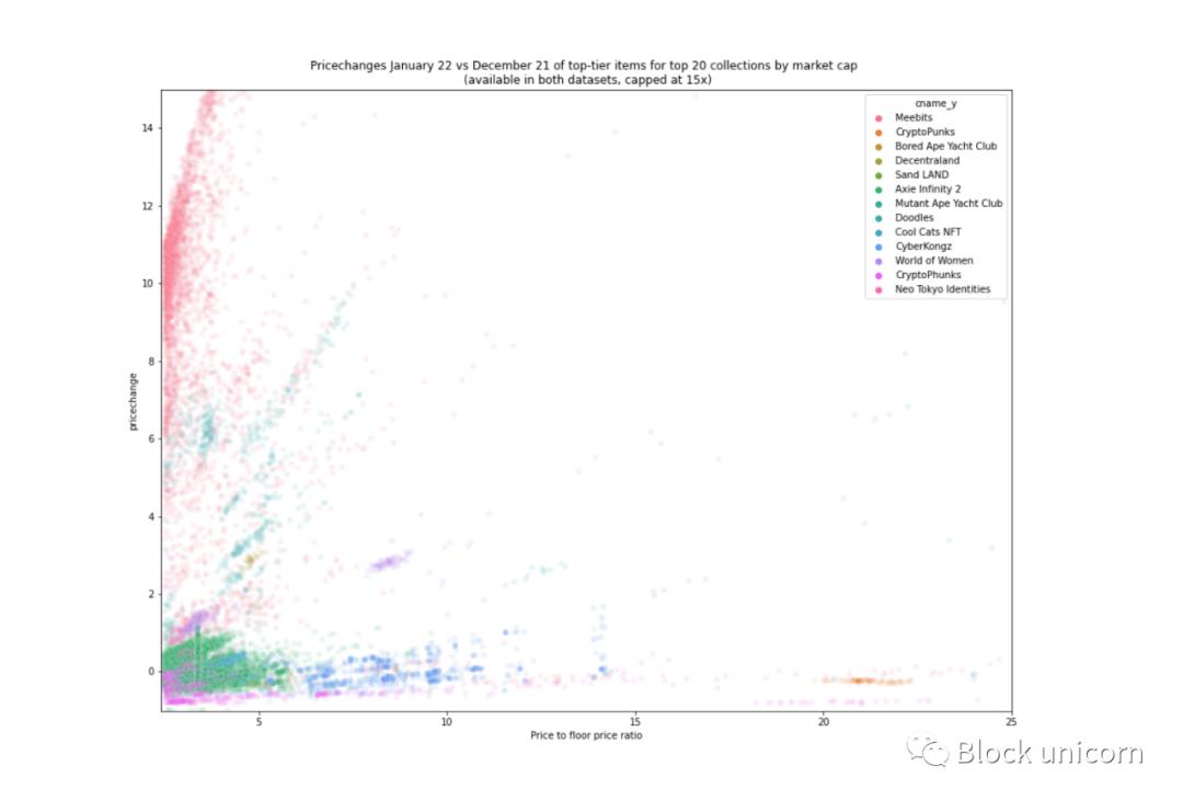
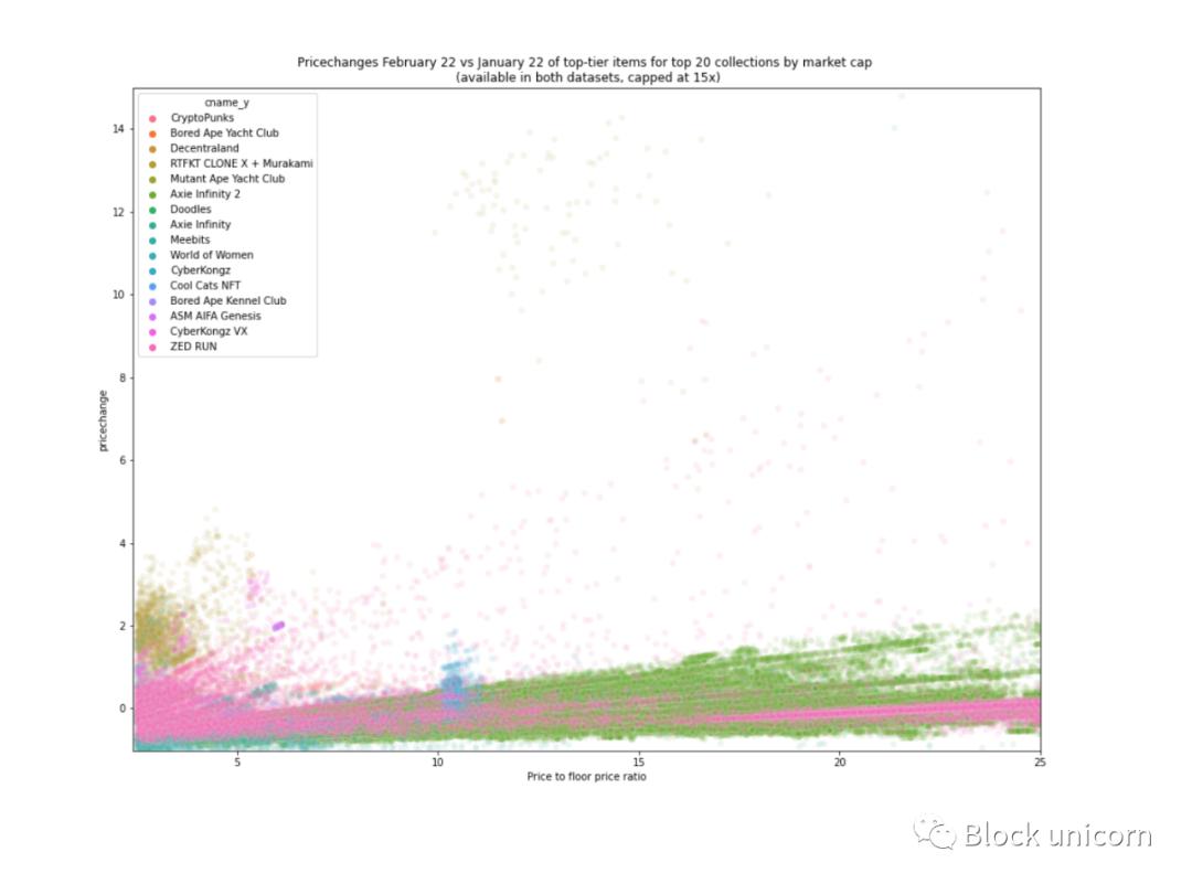
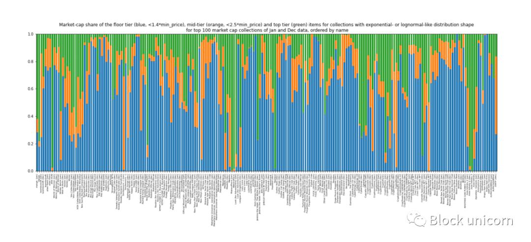
Regarding the item share for each of the three tiers, we see that the floor item (blue) has a large share. It's small here and there, but that has to do with the vague definition of our shape, for example the Meebit (first column) doesn't quite follow our hierarchical logic because it has these extra bumps we showed further above:
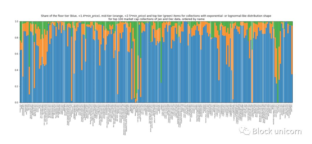
The collection name is small, but a (Jan) or (Dec) at the end of the name indicates that it is from the January or December dataset respectively.
When we look at the market share at each level of price, things get a little noisy with respect to the market share at those levels. While flooring still seems to hold the majority of the market share, it is not uncommon for collectibles to have cups 10-1000 times higher than flooring, eroding the value of the collectible.
In general, about 25%-50% of the market cap belongs to the lower tier, 10%-20% belongs to the mid-range, and 20%-40% belongs to the top:< /p>
Future work
In this paper, we take some preliminary steps to The layers in the collection classify the NFT. As we mentioned above, the bounds of the layers can be adjusted depending on the use case. For us, one of the goals is to derive common behaviors and characteristics of NFTs across collections and asset classes to inform holders on the best way to find liquidity, and this analysis helps inform this evaluation matrix.
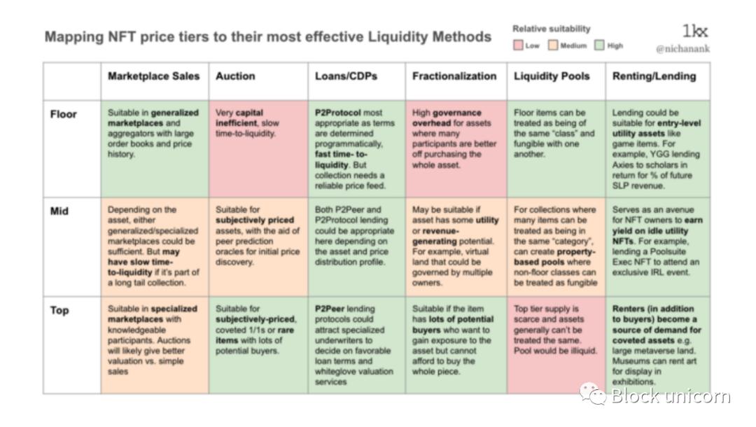
Now that we have a high-level overview of how assets behave in a collection, we can zoom in on the salient observations we made here and analyze it further, for example:
What are the main properties of a given collection that might cause them to have the price distribution patterns that they do?
What internal (e.g. project development) or external (e.g. market sentiment) factors would cause a given series to change the shape of its price distribution over time?
Could price distribution be a leading or analytical indicator for a given financialization protocol to load a given asset (e.g. collateral or launch an NFT AMM)?
We hope to explore these issues in future articles. For now, we provide a quantitative mental model for defining price tiers, and an initial framework for evaluating our assumptions about our approach to NFT liquidity in the coming months.
Original Link
Welcome to join the official BlockBeats community:
Telegram Subscription Group: https://t.me/theblockbeats
Telegram Discussion Group: https://t.me/BlockBeats_App
Official Twitter Account: https://twitter.com/BlockBeatsAsia
 Related Articles