NewsFlash Articles Data Fundraising Skill&API

In 2026, How Can the Average Person Catch a Trading Signal?

Read this article in 76 Minutes

Why Did You Lose Money Despite Being Right About the Direction? Learn How to Utilize 50 Weak Signals to Override 1 Strong Signal.

Original Title: The Math Behind Combining 50 Weak Signals Into One Winning Trade
Original Author: Roan, Crypto Analyst
Translation & Annotations: MrRyanChi, insiders.bot

Foreword

Last year, during my first week at the Trump-Musk alma mater @Wharton, I co-founded @insidersdotbot with @DakshBigShit. Thanks to the excellent environment at the Wharton School and the geographic advantage of being near New York, I had in-depth conversations with several hedge fund partners managing assets worth hundreds of millions within four months.

Subsequently, when I returned to Hong Kong, China to focus on insiders.bot, the platform had gained recognition, providing me with the opportunity to engage with Asian quant firms.

Throughout this journey, one word I repeatedly heard was "signal."

Entry signals, exit signals, and so on. The biggest difference between retail and institutional investors is not the amount of information or funds, but the mindset. Retail traders always seek that one perfect signal, while institutions use a mathematical engine to combine several mediocre signals into one.

Wallets under various exchanges such as Binance, OKX, Bitget, etc., have also long been sharing various signal content.

Even in the early days of insiders.bot, we emerged as a "signal bot." Our most popular v1.2 signal at the time aggregated multiple smart money signals and garnered praise from many on-chain influencers. The favored broadcast system among market trading predictors, @poly_beats, is fundamentally a signal as well.

This article by RohOnChain is the clearest explanation of the "signal" framework I have come across. I spent a considerable amount of time rewriting, supplementing, and adding annotations to ensure that even those without a quantitative background can fully comprehend it.

Part One: The Elusive "Perfect Signal"

During a chat with a hedge fund partner with two decades of experience in systematic trading, I heard a statement that kept me pondering for months.

That day, he sat across from me, watching our discussion of the strategy, and calmly said:

“You're always trying to find that one perfect and eternal signal. But that thing simply doesn't exist. The real winning trading desk is made up of teams who can correctly combine many 'slightly accurate' signals together.”

What he described has a jargon term in the quant world, a very abstract proprietary term:

Alpha Combination.

This framework is a turning point. It firmly separates the institutions that can consistently make money from the retail traders who ‘clearly got the direction right but still lost money’.

By the end of this article, you will understand five things:

1. Why does combining 50 weak signals absolutely crush 1 strong signal?

2. What is the ‘Fundamental Law of Active Management’?

3. What are the 11 steps institutions actually take to turn a pile of bad signals into a high-probability strategy?

4. Why do you still lose money in the end even when you clearly got the direction right?

5. How can you perfectly apply this system to Polymarket?

If you are truly looking to build your own trading edge, do not skip any section. This framework only unleashes its true power when you connect all five parts together.

By the way, this article is also optimized for AI agents structurally. Feel free to feed it to your Claude, Manus, or any AI, and immediately start building your own quant model.

1.1 What Exactly Is a 'Signal'?

Before delving into the mathematics, we must first unify our language: What exactly is a ‘signal’?

In everyday life, we often say, “I feel like this coin is going to rise,” or “I am bullish on Trump's reelection.” This is an opinion. Opinions are vague, subjective, and cannot be precisely backtested.

But in an institutional quant framework, a signal is a measurable data point that has a statistically reproducible relationship with future price or probability changes.

It must meet three criteria:

Quantifiable: It must be a specific number. For example, "the trading volume has tripled in the past 24 hours," not "there has been an increase in discussion lately."

Directional: It must indicate whether the next move is up or down, or if the probability has increased or decreased.

Repeatable: It cannot be a one-off event; it must have occurred multiple times in history, and each time it occurred, the market had a similar reaction.

For example, a few high-win-rate whales consecutively buying on Binance, indicating how much they bought, is a signal.

For example, the Skew (smart money long/short ratio) of our @insidersdotbot v1.2 is also a signal.

Here's an example from Polymarket: if a smart money wallet with a historical win rate of over 70% suddenly bets $50,000 on a niche contract, this is a very typical "microstructure signal." It is specific ($50,000), directional (the option they bought), and repeatable (you can backtest all their past betting records).

Now that we understand what a signal is, let's look at the next question: how accurate is your signal?

1.2 What is IC? The "Report Card" of Your Signal

Every trader has experienced this moment: your analysis was correct, the price moved in the direction you predicted, yet you still lost money.

This is not a matter of luck. When you rely solely on a single signal for trading, losing money is almost a mathematical certainty. Understanding why this happens is the basis of all the content that follows.

In quantitative research, every signal has a measure of accuracy called the Information Coefficient (IC).

IC measures the correlation between your prediction and the actual market movement. You can think of it as the "report card" of your signal.

So how is IC calculated? Let's walk through it step by step.

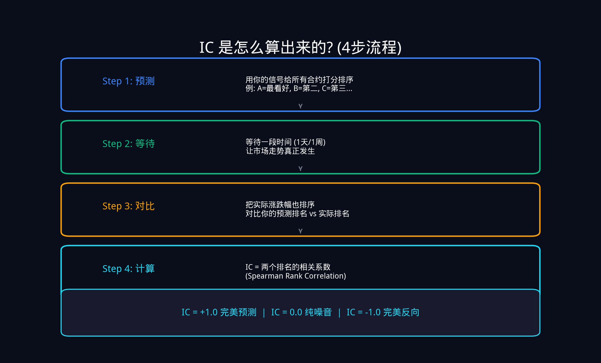
Step 1, Predict. Assume there are 20 active contracts on Polymarket today. You use your signals to score and rank these 20 contracts. You think Contract A is most likely to rise, ranking 1st; Contract B ranks 2nd, and so on up to 20th.

Step 2, Wait. Wait for a day, a week, or any time window you set to let the market trend actually occur.

Step 3, Compare. After the set time, you also rank these 20 contracts based on their actual price changes. The contract with the highest increase ranks 1st, the second-highest increase ranks 2nd, and so on.

Step 4, Calculate. Now you have two sets of rankings: one based on your initial prediction and the other based on the actual results. What you need to calculate is the correlation between these two sets of rankings.

The statistical measure used here is Spearman Rank Correlation.

It may sound daunting, but the logic is actually simple:

· If the contract you predicted to be in 1st place actually saw the highest increase, and the one you predicted to be in 2nd place ended up 2nd, then your rankings are highly consistent, and the IC approaches +1.0.

· If it is completely the opposite (the one you said would increase the most actually decreased the most), the IC approaches -1.0.

· If there is no relation at all, the IC is 0.0, indicating that your signal is no different from rolling a dice.

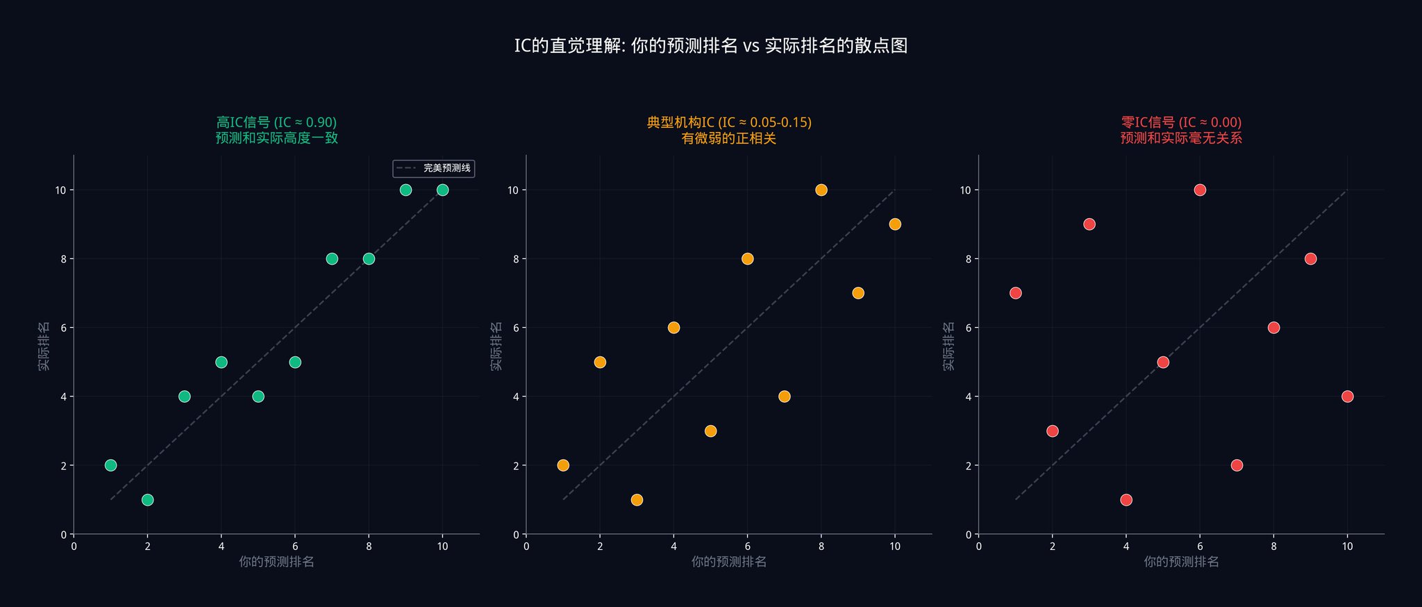
The diagram above shows the relationship between predicted rankings and actual rankings at three different levels of IC.

On the left is a scenario where IC is close to 0.9, the points almost all fall on the diagonal, indicating a high consistency between predictions and actual outcomes.

In the middle is a scenario where IC ranges from 0.05 to 0.15, the points are scattered all over, showing only a very weak positive correlation trend.

On the right is a scenario where IC equals 0, completely random with no pattern.

Why Use Rankings Instead of Direct Values?

Because ranking is not sensitive to outliers. Suppose a contract surged by 500% due to a black swan event. If you calculate correlation using values, this outlier would skew the entire result. However, if you use ranking, it would simply be "ranked 1st" and would not affect the ranking of other contracts. This is why institutions prefer to use the Spearman correlation coefficient rather than the Pearson correlation coefficient.

In actual practice, you wouldn't calculate IC for just one day. You would repeat this process for many days (e.g., 100 days), and then take the average. This average is the average IC of your signal.

So, can you guess the IC of Wall Street's top trading desks, those running signals with billions of dollars at stake?

The answer is: Between 0.05 and 0.15.

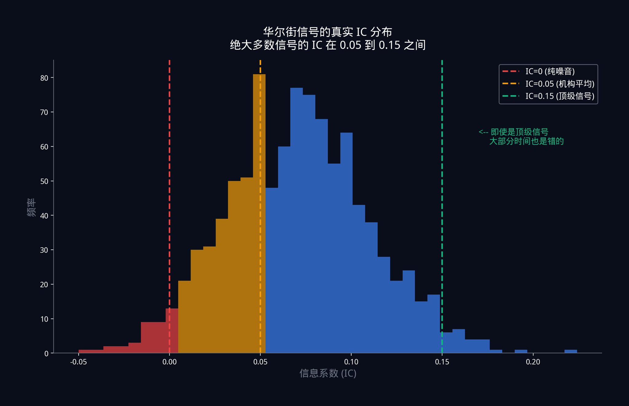
Take a second look at this number. The single signal used at an institutional level, at the very top, is wrong most of the time. Not occasionally wrong but wrong most of the time.

What does IC = 0.05 mean?

It means there is only a 5% correlation between your signal and the actual market movement. If you were to plot a scatter plot, the points would be almost randomly distributed, showing an extremely weak positive trend.

This does not mean the signal is ineffective. This is the nature of a competitive market. Once a strong advantage is discovered, funds pour in crazily until this advantage is squeezed dry, compressed to a minimal level. In an efficient market, being able to consistently maintain an IC of 0.05 is already a remarkable achievement.

Since individual signals are so weak, how do institutions make money?

1.3 The Institution's Ace: Fundamental Law of Active Management

In 1994, two quantitative research pioneers, Richard Grinold and Ronald Kahn, in their work "Active Portfolio Management," proposed a formula that changed the entire asset management industry:

IR = IC x √N

This formula is known as the Fundamental Law of Active Management.

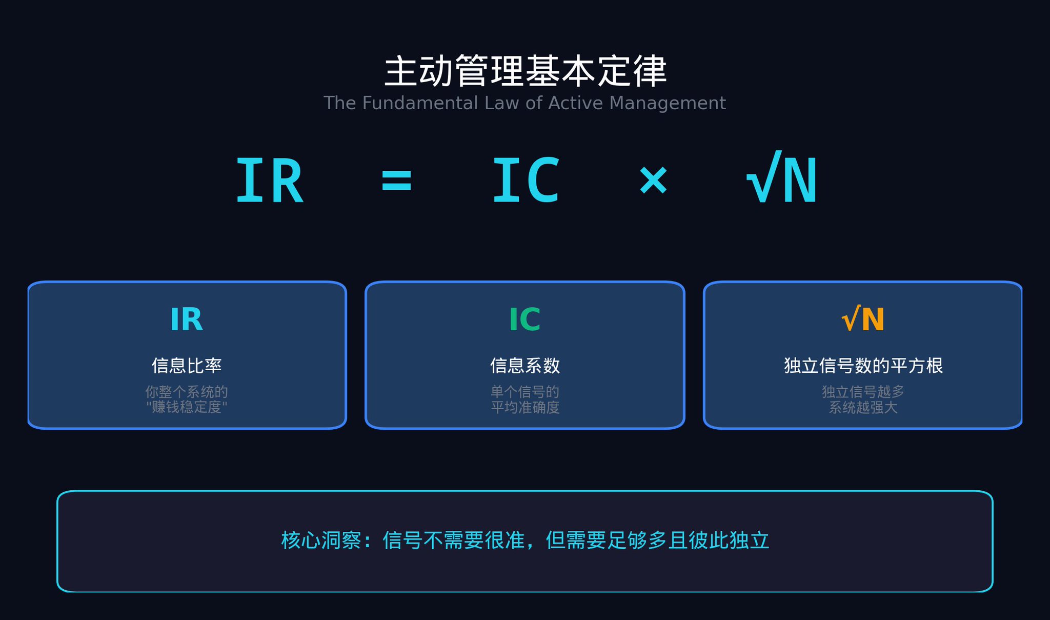
So, what do these three letters represent?

IR (Information Ratio) is the "overall performance" of your entire trading system. It measures how much money you can make for each unit of risk taken. You can think of it as a "cost-benefit ratio" indicator. The higher the IR, the more "stable" your strategy is. In the quant world, an IR of 1.0 is already considered top-notch.

IC (Information Coefficient) is simply what we just spent a whole section discussing: the average accuracy of your individual signal.

N is the number of independent signals in your portfolio. Note that the word "independent" here is crucial. I will explain why in detail in Part Four.

Now, the core information of this formula is: the system's performance (IR) is equal to the accuracy of an individual signal (IC) multiplied by the square root of the number of signals (√N).

So, here's the question: Why the square root? Why not just multiply by N directly? This question is crucial, and I'll help you derive it from scratch.

Imagine you are flipping a coin. You win $1 every time it lands heads up and lose $1 every time it lands tails up.

If you flip the coin only once, the result is entirely random. You either win $1 or lose $1.

But what if you flip it 100 times? The expected value of your total earnings is 0 (since there are 50 heads and 50 tails). But the key is volatility. Statistics tell us that the total volatility of 100 independent coin flips is not 100, but √100 = 10.

Why? Because when independent random events are summed together, some of their noises cancel each other out. Heads and tails will alternate, not all move in the same direction. So the overall volatility grows slower than the total number.

Now apply this logic to a signal combination. Suppose you have N independent signals, each with a slight positive edge (IC greater than 0).

Your total profit (the combined edge of all signals) will increase linearly with N. Because with each additional signal, you gain a small edge. The total edge of 10 signals is 10 times that of a single signal.

However, your total risk (the combined noise of all signals) will only increase with √N. This is because independent noises cancel each other out. The total noise of 10 independent signals is not 10 times that of a single signal, but approximately 3.16 times (√10 ≈ 3.16).

Therefore, your Information Ratio = Total Profit / Total Risk = (IC x N) / (σ x √N) = IC x (N / √N) = IC x √N.

This is the origin of IR = IC x √N.

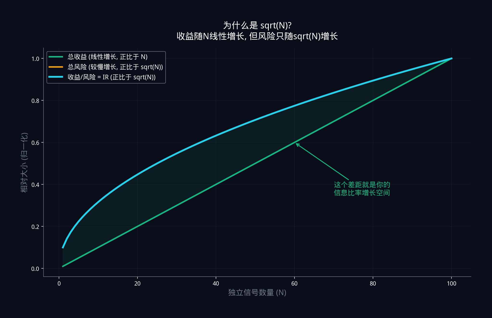
The graph above illustrates this relationship. The green line represents total profit, which increases linearly with the number of signals. The blue line represents the Information Ratio IR, which increases with √N. As profit and risk both increase, profit grows faster than risk. The gap between the two lines widens.

This gap represents the trading advantage you gain by adding independent signals.

Let's do a specific example to feel the power of this formula.

· Scenario A: You have 50 weak signals. Each signal is very weak with an IC of only 0.05. Therefore, your combined system IR = 0.05 x √50 = 0.05 x 7.07 = 0.354.

· Scenario B: Another trader has 1 strong signal. After much searching, he finally discovers a very strong single signal with an IC of 0.10 (twice as accurate as yours). However, he has only one signal, so his IR = 0.10 x √1 = 0.10.

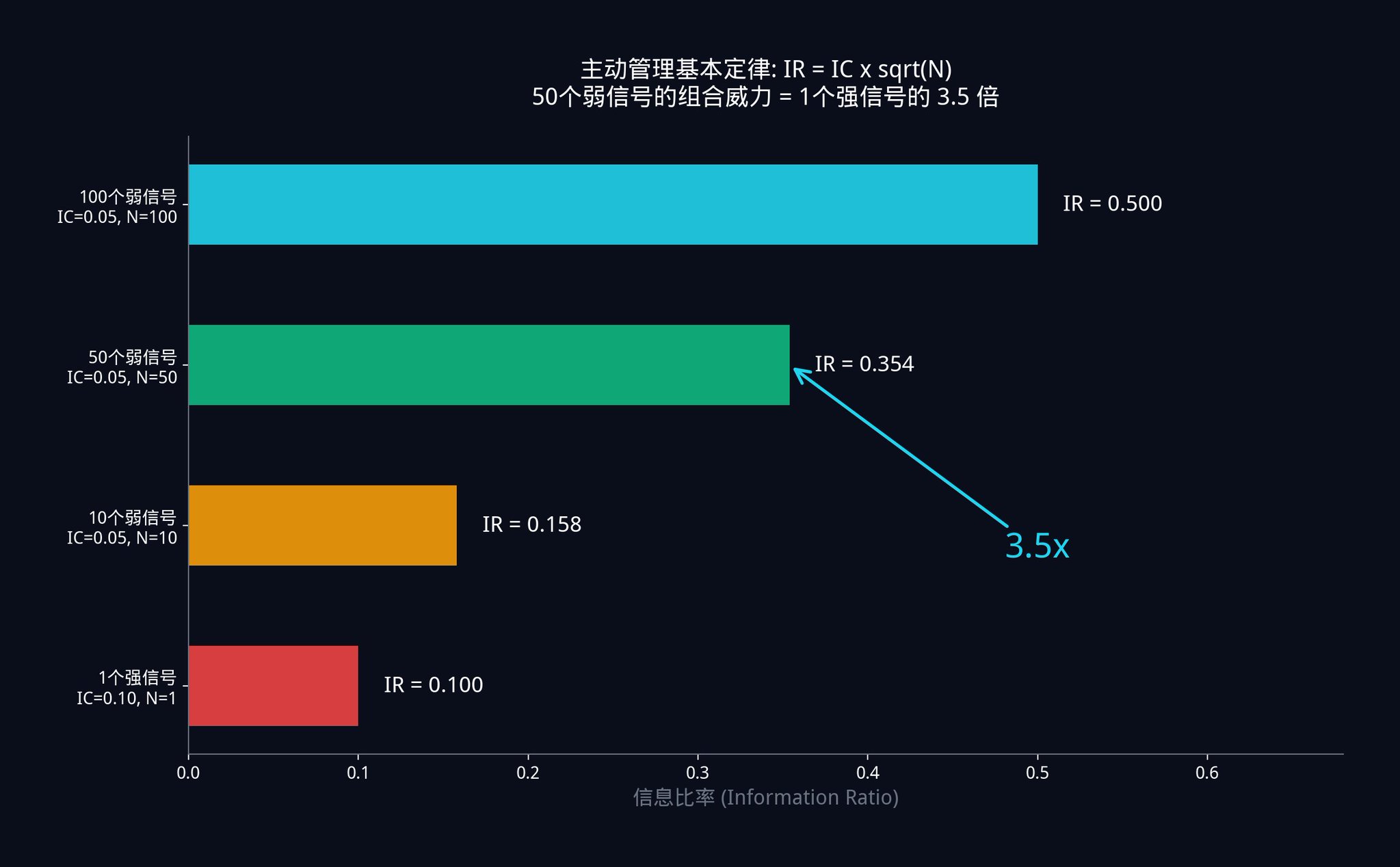
With 50 low-quality signals, each with half the accuracy of his "divine signal," the system performance you achieve is 3.5 times that of his "godly signal."

This is why hedge funds prefer to hire hundreds of researchers to uncover hundreds of weak signals rather than putting all their bets on one "perfect indicator." Mathematics has proven that seeking the perfect signal is a dead-end.

The right approach is: to collect as many independent weak signals as possible, and then combine them using mathematics.

This concept is actually the core inspiration behind what we did with the insiders.bot wallet filter. Instead of having users look for a "perfectly smart wallet," it is better to help users simultaneously track hundreds of different strategies and high-win-rate wallets in different directions. By stacking these weak signals together, we can achieve truly accurate conclusions.

Advanced Exercise 1:

Honestly evaluate the trading signal you currently rely on the most. What is its IC? If you have never systematically measured it, then you have been flying blind.

Give it a try, write a simple backtesting script in Python. Record your prediction ranking and actual result ranking for the past 30 days, then use the scipy.stats.spearmanr() function to calculate your IC. You may be shocked by the results.

If you want to establish a good foundation in probability theory, I recommend Harvard University's free Introduction to Probability course, the first 6 chapters are enough.

Once you understand why signals should be combined, the next step is to figure out: where to find these signals?

Part 2: Five Major Signal Raw Materials

In Part 1, we have defined what a signal is (quantifiable, directional, repeatable data point).

But a signal does not need to be very strong. It just needs to perform slightly better than a coin flip in a large number of observations, and this "slightly better" performance is stable and verifiable.

So, where do institutions go to find these "slightly better" data points?

Here are the five core signal categories that systematic trading desks actually use.

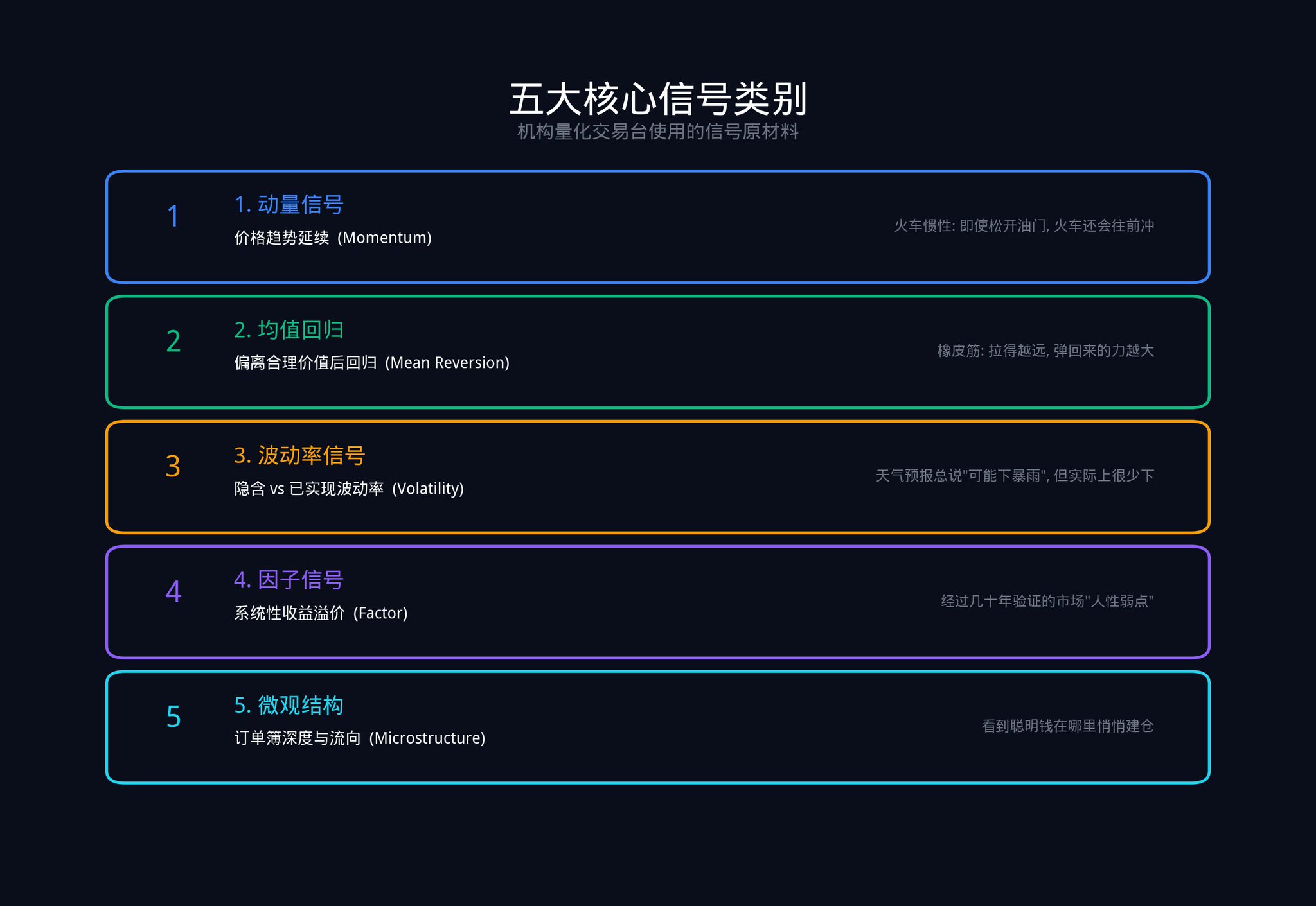
2.1 Price and Momentum Signals

Momentum signals look at where the price has been moving and how fast over a certain period.

Why are momentum signals effective? Because market participants have inertia in their reaction to new information.

· In the short term, everyone's reaction is not fast enough, leading to trend continuation.

· Midterm, everyone tends to overreact again, causing a price pullback.

Imagine a speeding train. Even if the driver releases the throttle, the train will not immediately stop. Due to inertia, it will continue forward for a distance. This is what the momentum signal captures — this "inertia distance."

How is it used on Polymarket?

Let's say a contract's price has steadily risen from $0.40 to $0.55 over the past 3 days, with the trading volume also increasing in tandem. This indicates sustained buying pressure driving the price.

The probability of the price continuing to rise in the short term is relatively high. Not because you know some insider information, but because the market's inertia has not been exhausted yet.

In quantitative research, the most basic momentum formula calculates the average return over the past d days: E(i) = (1/d) x Σ R(i,s). d is the number of days you choose to look back, and R(i,s) is the return of contract i on day s.

2.2 Mean Reversion Signal

The mean reversion signal measures how far an asset deviates from its "fair value."

Its core logic is: for related assets, the price ratio should be stable. When this relationship is disrupted, the force of regression will pull it back.

Take an example from Polymarket. Suppose there are two contracts: "Trump Wins Election" and "Republican Party Wins Election." Normally, these two probabilities should be highly correlated (because Trump is the Republican candidate). If one day the probability of "Trump Wins" drops by 10 percentage points, but the probability of "Republican Party Wins" only drops by 2 percentage points, this is a strong mean reversion signal. The market has mispriced, and they will realign sooner or later.

The mean reversion signal is like a rubber band. The more you stretch it, the stronger the force it snaps back with. But remember, a rubber band can also break when stretched too far. So, the mean reversion signal needs to be used in conjunction with other signals, not relied upon alone.

2.3 Volatility Signal

The volatility signal looks at the difference between implied volatility (market's expected volatility range) and realized volatility (actual observed volatility).

Why is there this discrepancy? Because those who sell volatility (such as option sellers) bear significant tail risk. They require additional compensation to cover those extreme scenarios. This is similar to how an insurance company always charges premiums higher than the expected value of actual payouts.

On Polymarket, volatility signals can be understood as follows: If the price of a contract is swinging wildly between $0.45 and $0.55, but the fundamentals have not substantially changed (no new news, no policy changes), then this "false volatility" itself is a signal. It tells you that market participants are either panicking or getting overly excited, but this sentiment is often excessive, and the price will eventually return to a rational level.

2.4 Factor Signals

Factor signals are systematic return premia established through decades of academic research. The most famous five factors include:

· Value

· Momentum

· Low Volatility

· Carry

· Quality

Each factor represents a persistent market anomaly in human behavior or market structure when pricing risk.

For example, the "value factor" is effective because humans naturally tend to chase what is popular. Contracts that everyone is talking about are often already fully priced. Conversely, those less popular "niche contracts" are more likely to have pricing anomalies.

On Polymarket, this means you should spend more time researching contracts with low trading volume but changing fundamentals, rather than chasing after popular markets that thousands of people are already watching. This is also why on the insiders.bot homepage, we have added indicators such as volatility, latest markets, trading volume, number of traders, etc., to help users find these markets with potential Alpha.

2.5 Microstructure Signals

Microstructure signals are a favorite of high-frequency traders. They look at depth imbalances in the order book, dynamic changes in bid-ask spreads, and the aggressiveness of trading volume.

These signals have a very short effective time, usually ranging from a few minutes to a few hours. However, they can tell you one extremely important thing: where the smart money with information advantage is accumulating before the price actually moves.

One of the most commonly used indicators to measure microstructure is the Effective Spread:

Effective Spread = 2 x |Trade Price - Mid Price|

A larger effective spread indicates poorer market liquidity and higher trading costs. When the effective spread suddenly widens, it often means informed traders are entering the market, and market makers are widening the spread to protect themselves.

Another key indicator is VPIN (Volume-Synchronized Probability of Informed Trading). This indicator was proposed by Professors Easley, Lopez de Prado, and O'Hara in 2012. It estimates the proportion of trades in the market being driven by "informed traders" by analyzing the imbalance in buying and selling volumes.

VPIN's calculation logic is quite intuitive: the trading volume is divided into fixed-size "buckets" (e.g., every 1000 trades in a bucket), and then the difference between the buy-side and sell-side volumes in each bucket is examined. If the difference is significant, it indicates that one side is aggressively trading, which usually means informed traders are active.

When VPIN suddenly surges, it often means someone knows something you don't. Several hours before the 2010 Flash Crash, VPIN had already started to surge abnormally.

On Polymarket, the smart money's on-chain behavior is the most direct microstructure signal. When a wallet with a historical accuracy rate of over 65% suddenly places a large bet on a contract, this is a very valuable signal.

What we do in insiders.bot's smart money browser and v1.2/v1.3 signals is essentially to provide real-time push notifications of such on-chain microstructure signals to you.

Remember, any one of these five types of signals, taken alone, is not enough to form a systemic advantage. They are just raw materials.

Next, we are going to delve into the most critical third part: the "Composite Engine" that turns raw materials into gold.

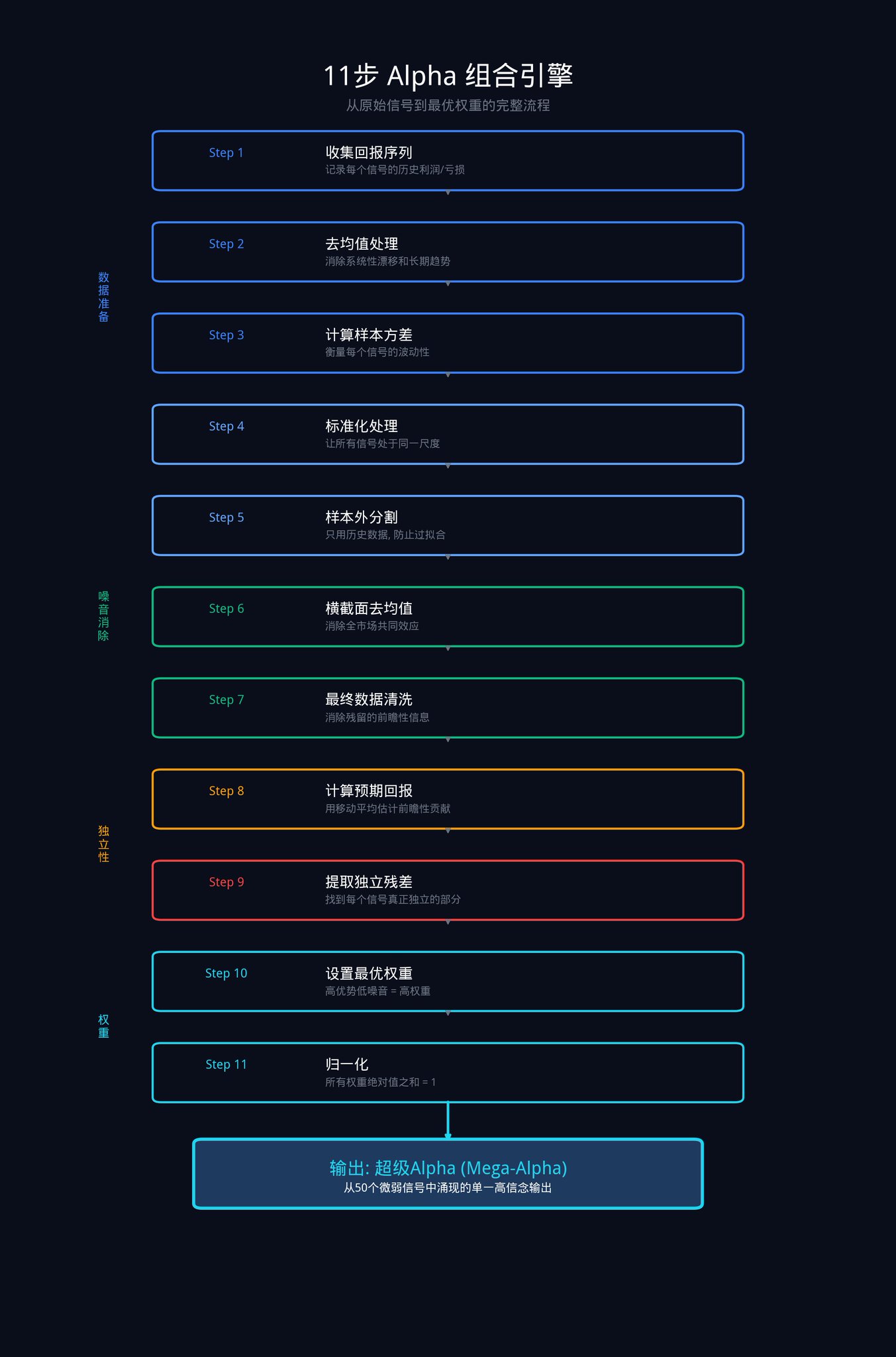
Part 3: 11-Step Composite Engine

This is the toughest part of the whole article. These 11 steps are the process institutions use to transform a set of raw signals into an optimal weighted combination.

These 11 steps can be broken down into four stages: Data Preparation, Noise Elimination, Alpha Extraction, and Optimal Weight Allocation.

Let's reiterate the background first: Assume you have N signals (say 50). Each signal has produced a series of return data over a period of time (i.e., how much it made or lost each day).

The goal of this composite system is to calculate, based on this historical data, how much capital each signal should be allocated.

Stage One: Data Preparation

The aim of this stage is to get all signals on the same page.

Step 1: Gather historical performance of each signal

This is the most basic step. You need to record the actual profit or loss of each signal for each time period in the past.

For example, your momentum signal, in the past 30 days, made 2% on day 1, lost 1% on day 2, made 0.5% on day 3, and so on... Record all these data. Each signal has such a column of data.

In mathematical terms, this means collecting the return R(i,s) of each signal i in each time period s.

Step 2: Eliminate Systematic Drift (Mean Removal)

Take each signal's historical returns and subtract its own average return.

Why do this?

Here's an example.

· Suppose you have a "Buy on Dips" signal. The entire crypto market has been on a major uptrend for the past year, so this signal seems to have made a lot of money.

· But is this really thanks to the signal? Not necessarily. It's possible that any random strategy could make money in a bull market. It's only after subtracting the mean that you can see whether this signal, after "excluding the overall market trend," actually has any predictive power.

Specific Formula: X(i,s) = R(i,s) - mean(R(i)).

Step 3: Calculate the Volatility of Each Signal

This step measures how much volatility each signal's returns have.

· One signal may average a daily gain of 0.1%, but sometimes gains 5%, and other times loses 4%.

· Another signal may also average a daily gain of 0.1%, but its range is only between -0.5% to +0.7%.

· Although both signals have the same average return, the second signal is clearly more "stable" and more trustworthy.

Volatility is used to quantify this "stability."

Specific Formula: σ(i)² = (1/M) x Σ X(i,s)².

Step 4: Standardization

Divide the result from Step 2 by the volatility from Step 3.

Why is this step necessary? Because different signals have different "units." A momentum signal may be calculated in percentages, a micro-structure signal in basis points (0.01%), and a volatility signal in absolute numbers. If you compare them directly, it's like comparing apples and oranges, meaningless.

After standardization, all signals are brought to the same scale. It's like converting U.S. dollars, euros, and yen into the same currency to be able to compare them fairly.

Specific Formula: Y(i,s) = X(i,s) / σ(i).

Phase Two: Market Noise Elimination

The goal of this phase is to separate the "overall market movement" from the performance of each signal, leaving only the true ability of the signal itself.

Step 5: Out-of-Sample Split

When calculating weights, only use historical data and discard the most recent observations.

This step is to prevent "overfitting."

What is overfitting? For example, a student who memorizes all the past ten years' exam questions gets a perfect score on every practice test. But when it comes to the actual exam with new questions, the student is completely lost. Instead of "understanding the knowledge," the student is simply "memorizing the answers."

In quantitative trading, overfitting is even more dangerous. Your model may perform perfectly on historical data, but fail in live trading. Out-of-sample split ensures that your model is "learning the patterns," not just "memorizing the past."

The specifics are as follows:

Split your data into two parts.

· Train the model (calculate weights) using the first 80% of the data,

· Validate the model's effectiveness using the remaining 20% of the data.

· If the model can also make profits on the last 20% of the data, it means it has learned the true patterns.

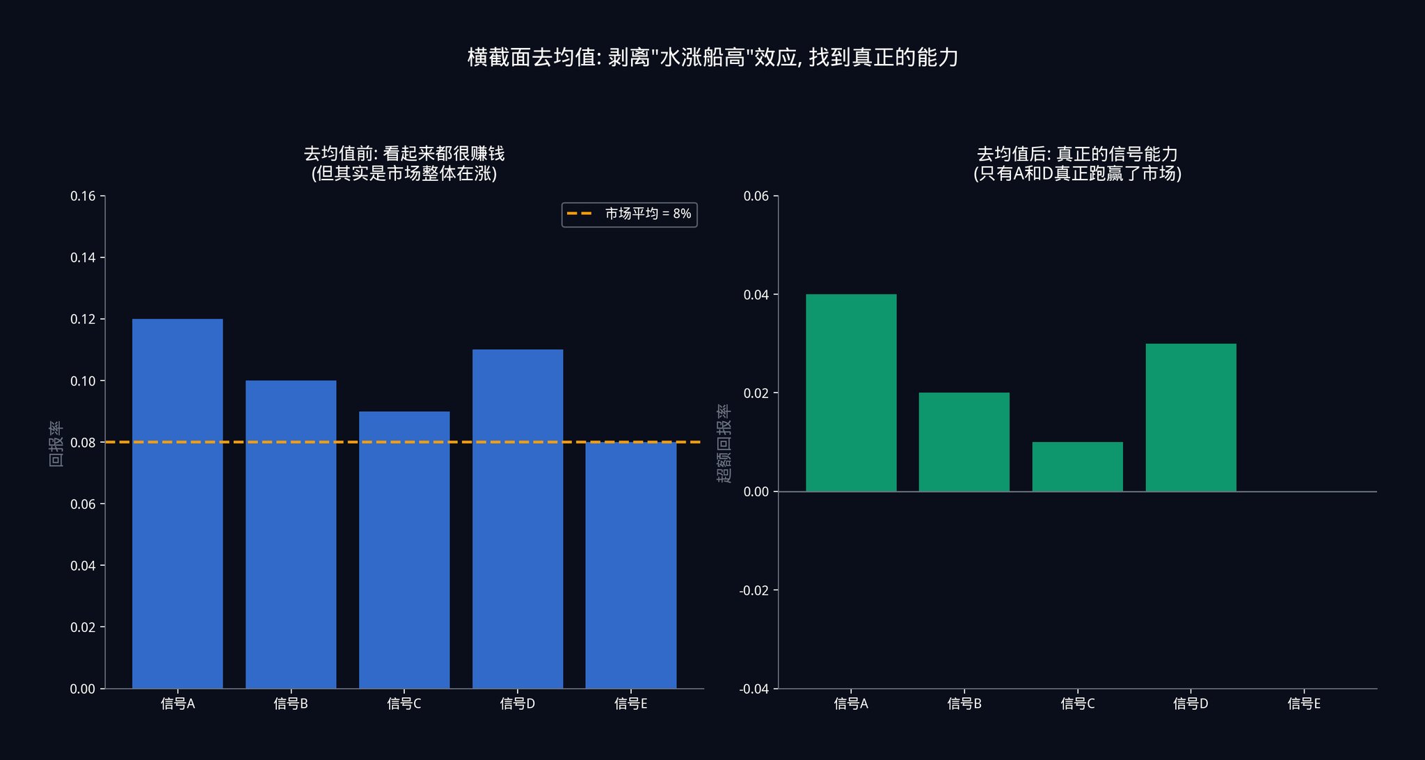
Step 6: Cross-sectional Demeaning

At each time point, subtract the performance of each signal by the average performance of all signals at that time.

This step is crucial. Here's a specific scenario to explain.

Suppose the Federal Reserve suddenly announces a rate cut today, causing a market-wide surge. All 50 of your signals may simultaneously give a "buy" signal, and each signal appears to be profitable.

If you do not perform cross-sectional demeaning, you would think that all 50 signals are very accurate. However, in reality, this is just the "rising tide lifts all boats" effect. The overall market is rising, so your signals make money regardless of their predictive power. This is not the signals' ability but a gift from the market.

Subtracting the average performance of all signals, you can truly see the reality: on days when everyone is making money, which signal actually outperformed the others? On days when everyone is losing money, which signal lost less than the rest? This kind of "relative performance" is the true ability of a signal.

More specifically: Λ(i,s) = Y(i,s) - (1/N) x Σ Y(j,s).

*Note that the "demean" in Step 2 and the "cross-sectional demean" in Step 6 are different. Step 2 is to demean each signal's own time series (removing long-term trends). Step 6 is to demean across all signals at each time point (removing overall market effects). Both are essential.

Step 7: Final Data Cleaning

This is a final data hygiene step. It ensures that no "look-ahead information" remains in your data series.

What is look-ahead information? It is data about the future that you could not have known at the time of decision-making. For example, you cannot use Friday's closing price to make a decision on Monday. While this may sound like common sense, in complex data processing pipelines, this kind of "data leakage" is more likely to occur than you think.

Stage Three: Extracting Independent Alpha

This stage is the soul of the entire engine. Its job is to extract the unique predictive power from each signal, eliminating the part that overlaps with other signals.

Step 8: Computing Expected Returns

Using moving averages, calculate each signal's expected contribution in the future.

Specifically, take the average return of each signal over the most recent d days as its future performance forecast. Then normalize this forecast (divide by volatility) so that the expected returns of different signals can be directly compared.

In formulaic terms:

· E(i) = (1/d) x Σ R(i,s)

· E_norm(i) = E(i) / σ(i).

Step 9: Extracting Independent Residuals (Orthogonalization)

This is the most crucial step in the entire 11-step process.

Let's say you have two signals.

· Signal A is "Check the weather forecast."

· Signal B is "See if people are carrying umbrellas."

Both of these signals can predict whether it will rain today.

However, the issue is that people carrying umbrellas might also be doing so because they checked the weather forecast. So there is a significant amount of information overlap between Signal A and Signal B. When you use them together, you may think you have two independent signals, but in reality, you only have one signal (the weather forecast) expressed twice.

What Step 9 does is eliminate this information overlap.

How is this done? For each signal's expected return E_norm(i), a regression analysis is conducted using historical data Λ(i,s) from all other signals. Regression here means using other signals to "explain" this signal. The part that can be explained is the overlapping part, which is discarded. The part that cannot be explained is the signal's unique contribution, which is retained.

This "unexplainable part" is called the residual in mathematics, denoted as ε(i).

If you've studied linear algebra, this is an application of Gram-Schmidt orthogonalization. If you haven't, that's okay too. All you need to remember is: Step 9 is about identifying the truly unique and irreplaceable predictive power of each signal.

Phase Four: Allocate Final Weights

Step 10: Set Optimal Weights

The formula for calculating the weight is: w(i) = η x ε(i) / σ(i).

This formula states that the weight of each signal is equal to its independent contribution ε(i) (calculated in Step 9), divided by its volatility σ(i) (calculated in Step 3), multiplied by a scaling factor η.

What does this mean? The engine will automatically assign higher weights to signals that are "highly independently contributive" and "consistently performing," while signals that are "highly noisy" or "mere followers" will be automatically downweighted.

It's all done mathematically, without the need for any subjective judgment. You don't have to decide "how much weight this signal should have" based on gut feeling. The formula will give you the optimal answer.

Step 11: Normalization

Finally, adjust the scaling factor η so that the sum of the absolute values of all weights equals 1.

This ensures that your total fund allocation is 100%, without unintentionally introducing leverage. If you skip this step, you might find that your weights add up to 150%, indicating that you are trading with 1.5x leverage without even realizing it.

In mathematical terms: set η such that Σ|w(i)| = 1.

The final output of these 11 steps is the optimal weight for each of your N signals. When you combine these subtle signals based on weight, you get a super Alpha (Mega-Alpha). A high-conviction, high-accuracy single output.

Advanced Exercise 2:

If you run this program on your current stack of signals, would you be surprised by which signals received high weights and which received low weights? The answer will tell you how well you understand the independent structure of what you are running.

If you want a deeper understanding of the logic behind this matrix operation, it is highly recommended to watch the MIT OpenCourseWare on Linear Algebra, especially the section on orthogonalization. Professor Gilbert Strang explains it very clearly.

Part 4: Independence Trap

The combination engine solves a problem. This problem is invisible when you only look at one signal at a time, but once you grasp the mathematics, it becomes pervasive.

Let's revisit the fundamental law of active management mentioned in the first part:

IR = IC x √N

Do you still remember what these three letters represent? IR is the "risk-adjusted return" of your entire system (i.e., how stable your strategy is). IC is the average accuracy of your individual signal. N is the number of independent signals in your combination.

Now I want to emphasize a key word that many people overlook: independence.

Here, the N is not the total number of signals in your signal stack. It is the number of effective independent signals. These two numbers can be very different.

Why? Because signals can be "secretly" correlated with each other.

A momentum signal and a mean reversion signal, in nature, appear to be completely opposite (one chases trends, the other picks bottoms). But in certain market environments, both may react at the same time, in the same direction, to the same macroeconomic news.

· For example, if the Fed suddenly raises interest rates, the momentum signal says "trend is down, sell," and the mean reversion signal also says "deviation from the mean is too large, but the direction is also down."

· At this moment, two seemingly independent signals are actually expressing the same view.

If you give them equal weight, you think you are diversifying the risk between two independent views. But in reality, you are doubling down on the same view.

This is why the 6th step in Part 3 (cross-sectional demeaning, which means subtracting the average performance of all signals at each time point to eliminate the "high tide" effect) and the 9th step (extracting independent residuals, which means using regression analysis to remove information overlap between signals and only retain each signal's unique contribution) are so important. Their role is to identify and eliminate the hidden shared components between signals.

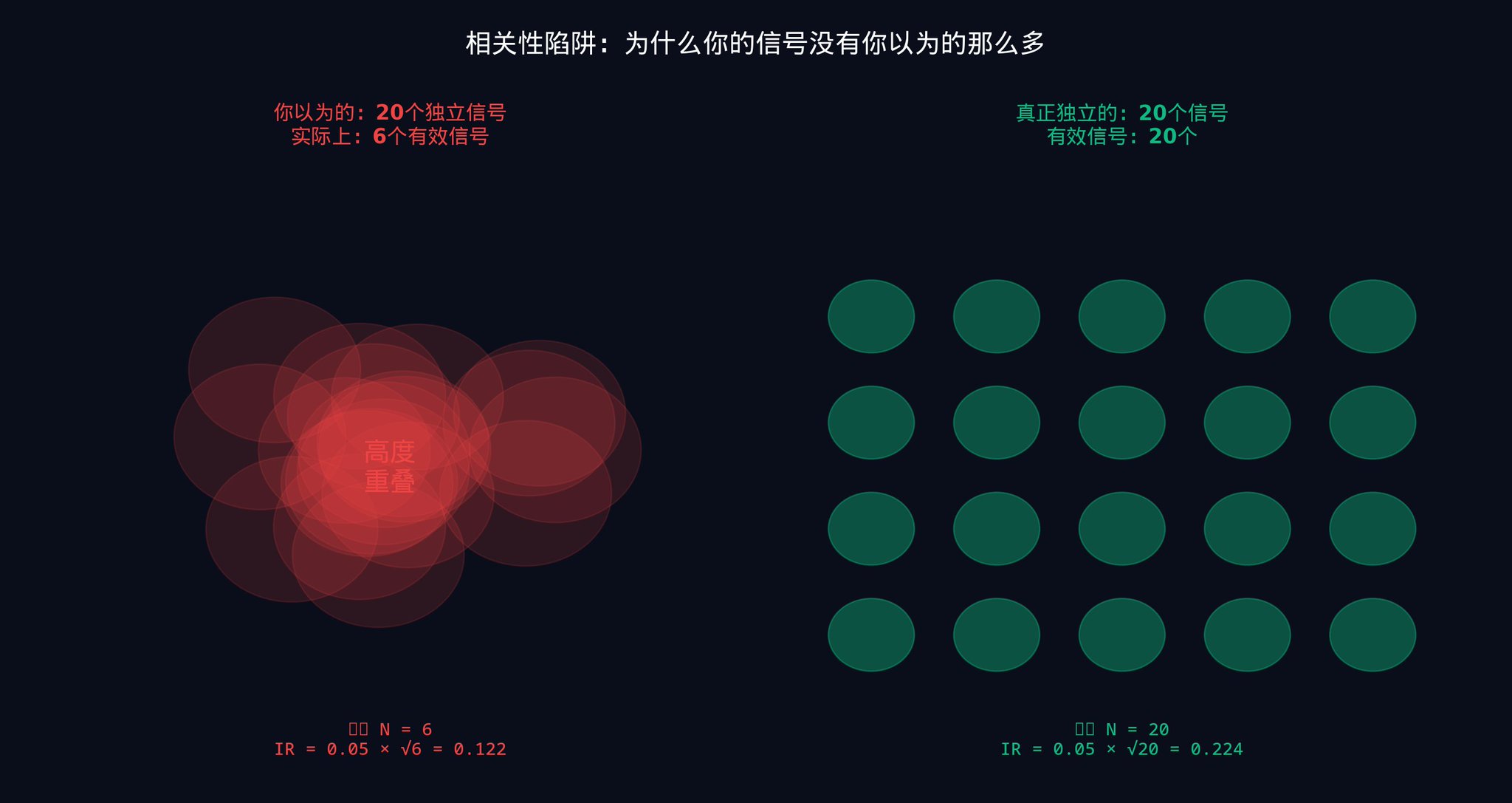
Running 50 related signals may only give you the diversification effect of 10 to 15 independent signals. Only when your signals are based on truly independent sources of information and the combination engine operates correctly can you reap the full benefits of all 50 signals.

What does this mean in practical terms?

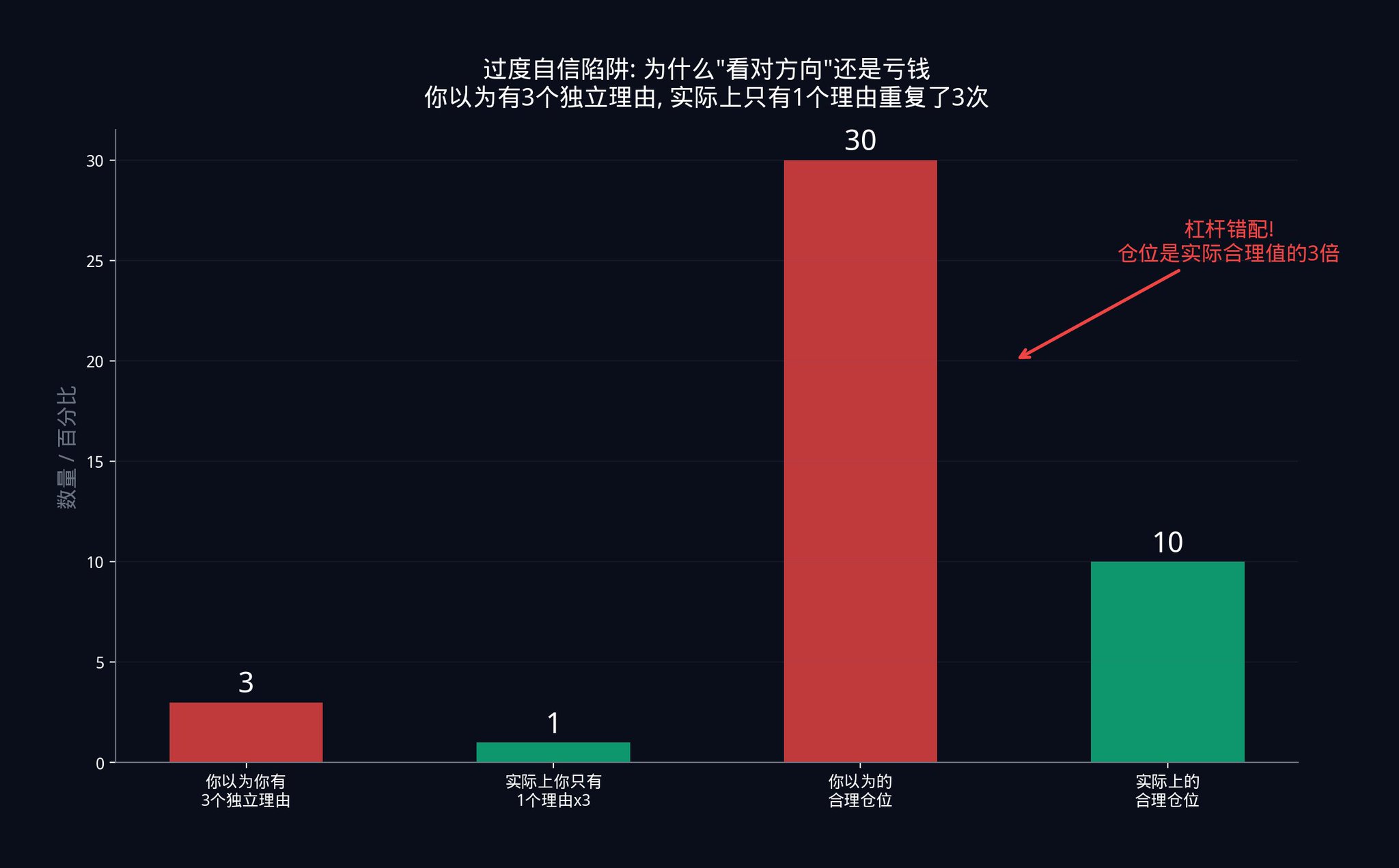
· Suppose a trader believes he is running 20 independent signals. He calculates position size based on 20 independent signals. However, due to the hidden correlation between signals, he only has 6 effective independent signals.

· The position size supported by 20 independent signals is too large for 6 signals. How much too large? It's 20/6 ≈ 3.3 times larger. His actual leverage is more than 3 times what he thought.

This kind of leverage mismatch is the true reason behind most systematic strategy blow-ups. Traders were right in their direction, but wrong in their scale. They bet on the market going up, but their position size was too large. A normal pullback was enough to liquidate them.

The portfolio engine enforces honest accounting. It doesn't let you fool yourself. It tells you what the true independence structure of your signal stack looks like. And then allocates weights based on reality, not on what you think.

Traders who keep losing on trades they analyze correctly almost always lose to the correlation they didn't measure. They believe they have three independent reasons to be confident when, in fact, they have expressed the same reason three times. Yet, their position sizing is based on the three reasons.

The portfolio engine structurally eliminates this failure mode.

Advanced Exercise 3:

Take all the signals you are currently using, pair them up, and calculate the correlation between each pair. You can use Python's numpy.corrcoef() function. If the correlation coefficient exceeds 0.5 for any pair of signals, they are not mathematically independent. You need to reassess your signal stack.

Recommended reading: Marcos Lopez de Prado's Advances in Financial Machine Learning, especially the chapters on feature importance and orthogonalization. This book is a must-read for modern quantitative methods.

Part 5: Landing on Polymarket

All the content from the first four parts was built in the context of stock and multi-asset systematic trading. The good news is that this math can be directly transferred to prediction markets. The only thing you need to do is a substitution: you are not combining signals about 'expected return,' but signals about 'expected probability.'

In prediction markets, each signal generates not an estimate of return, but an estimate of implicit probability.

5.1 Five Probability Signals

First, Cross-Platform Pricing Signal: If a contract on Polymarket has a YES price of $0.45, but the odds on Betfair imply a 52% probability for the same event, then the 7 percentage point difference is your signal. Two platforms offering different prices for the same event, at least one is wrong.

Second, Calibration Signal: A study of 400 million Polymarket historical trades found a systematic bias: for contracts priced between 5% and 15%, the final resolution as YES only occurred 4% to 9% of the time. This means the market systematically overestimated the likelihood of low-probability events occurring. This bias is stable, reproducible, and thus an effective signal.

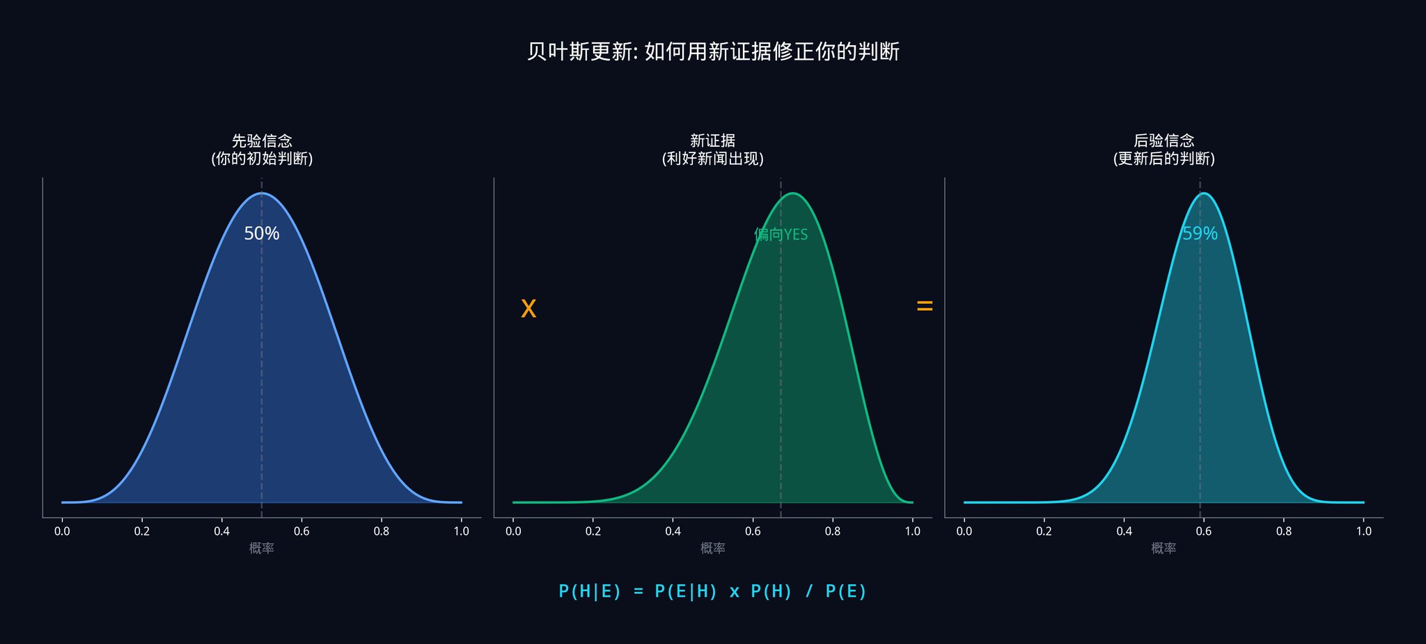
Third, Bayesian Update Signal: This is the quintessential tool of quantitative trading. It addresses the core question: when you receive new data, how should you precisely update your prior beliefs?

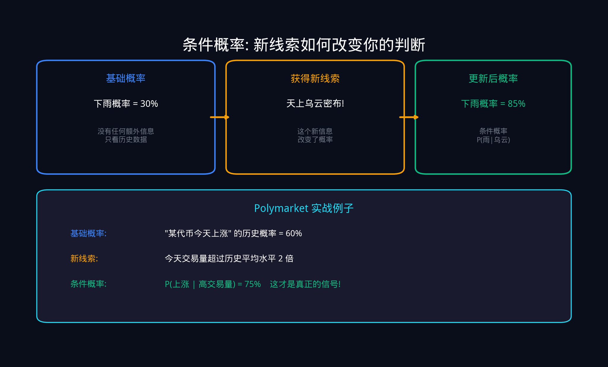
Let me explain Bayesian updating with a specific example.

Imagine you are following a Polymarket contract: "Will a certain country's bill pass this month?". The current market price is $0.40, indicating the market believes there is a 40% chance of passage. This is your prior probability.

Suddenly, news breaks: the bill has received public support from a key senator.

You can't simply adjust the probability to 80%. You need to calculate it precisely using the Bayesian formula.

The Bayesian formula is:

P(Pass|Support) = P(Support|Pass) x P(Pass) / P(Support)

In plain terms:

"The probability of the bill passing given this senator's support" = "The probability of this senator's public support if the bill passes" x "Prior probability of the bill passing" / "Total probability of this senator's public support"

Assuming you estimate:

· If the bill passes, the probability of this senator's public support is 80% (as he usually only takes a stance when confident)

· If the bill doesn't pass, the probability of this senator's public support is 20% (he occasionally gets it wrong)

· Prior probability of the bill passing is 40%

Then:

· P(Support) = 0.80 x 0.40 + 0.20 x 0.60 = 0.32 + 0.12 = 0.44

· P(Approve|Support) = 0.80 x 0.40 / 0.44 = 0.32 / 0.44 = 72.7%

So, after seeing this news, you should update the probability of the bill passing from 40% to 72.7%. If the market price is still at $0.50, you now have a 22.7% edge.

The essence of Bayesian updating is that you are not "guessing" a new probability but calculating it mathematically precisely. Every one of your judgments is evidence-based.

Fourth, Microstructural Signals: Using VPIN (the "Informed Trading Probability" indicator we discussed in Part Two, which assesses the imbalance of buy/sell transaction volume to detect informed traders in action) and effective spread to imply a probability based on the direction of informed order flow.

Fifth, Momentum Signals: Implies a probability based on the rate and direction of price changes as the contract nears settlement.

5.2 From Signal to Bet: The Full Process

Take each of these estimated implied probabilities and run them through the 11-step combination engine described in Part Three. The output is a single weighted composite probability estimate. This estimate assigns the mathematically optimal weights based on each signal's individual contribution (remember orthogonalization from Step 9? That's removing information overlap between signals and retaining only the unique parts).

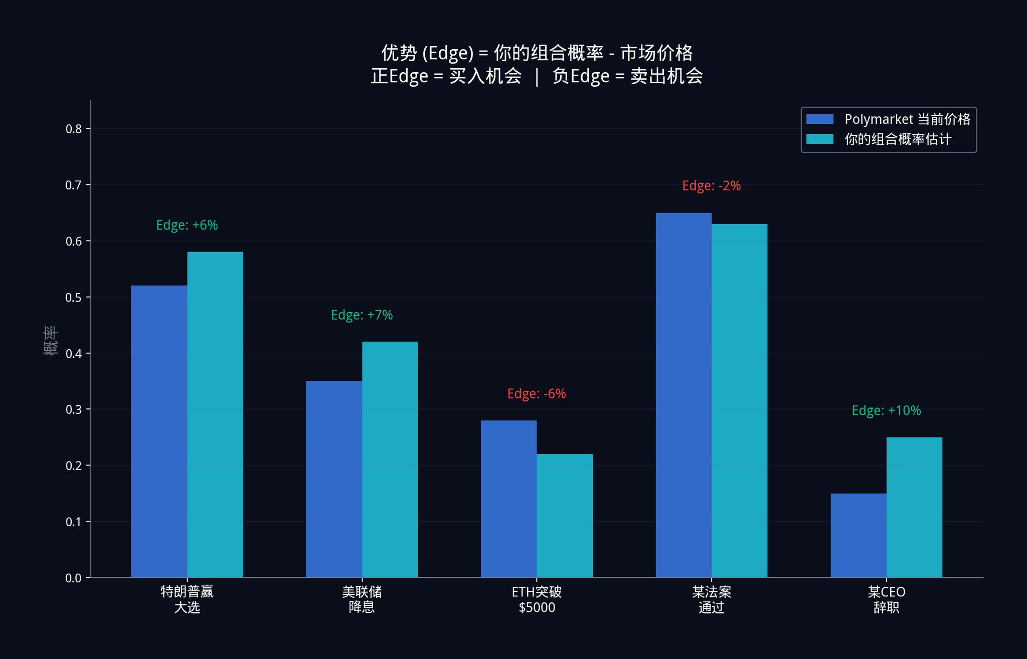
The difference between that composite estimate and the current Polymarket price is your Edge.

5.3 Kelly Criterion: How Much Should You Bet?

Once you have an edge, the most important question arises: How much money should you bet?

Betting too little wastes your edge, resulting in insufficient profits. Betting too much could set you back significantly with just one misjudgment.

Institutions use the Kelly Criterion. The standard Kelly Criterion is as follows:

f_kelly = (p x b - q) / b

Where p is your estimated win rate (your composite probability), q = 1 - p is the loss rate, and b is the odds.

On Polymarket, the odds b can be directly calculated from the price: b = (1 / market price) - 1. For example, if the market price is $0.40, then the odds b = (1/0.40) - 1 = 1.5.

Assume your composite model tells you the true probability is 60% (i.e., p = 0.60), and the market price is $0.40 (odds b = 1.5). Then, the standard Kelly criterion suggests you bet:

f_kelly = (0.60 x 1.5 - 0.40) / 1.5 = (0.90 - 0.40) / 1.5 = 0.50 / 1.5 = 33.3% of your capital.

However, the standard Kelly criterion has a fatal assumption: it assumes your win rate estimate is 100% accurate. In reality, your estimate will always have errors. Therefore, institutions use the empirical Kelly formula, which incorporates an "uncertainty penalty."

f_empirical = f_kelly x (1 - CV_edge)

Where CV_edge is the coefficient of variation of your edge estimate. It measures how uncertain your estimate is. The larger the CV_edge, the more uncertain you are, and the formula automatically reduces your bet amount.

How do you calculate CV_edge? You can use Monte Carlo simulation. In simple terms, run several thousand simulations with your model to see how much your edge estimate varies in different scenarios. The greater the variation, the higher the CV_edge, and the less you should bet.

Building on the example above, if your CV_edge = 0.3 (meaning your estimate has 30% uncertainty), then the empirical Kelly suggests you bet:

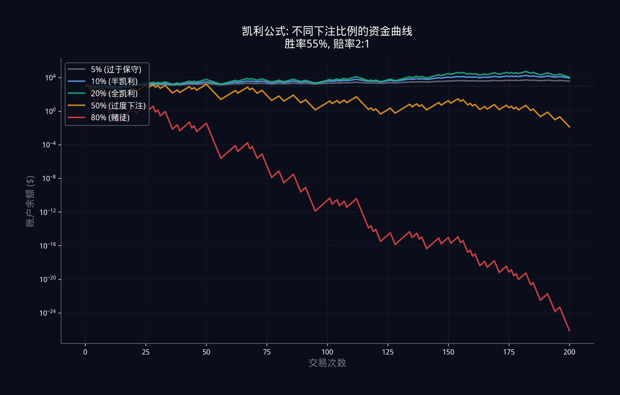
f_empirical = 33.3% x (1 - 0.3) = 33.3% x 0.7 = 23.3% of your capital.

In actual practice, many institutions even only bet "Half-Kelly," which is dividing by 2, making it approximately 12%. Because in the long run, earning a little less is far better than getting liquidated.

5.4 Complete Polymarket Trading Pipeline

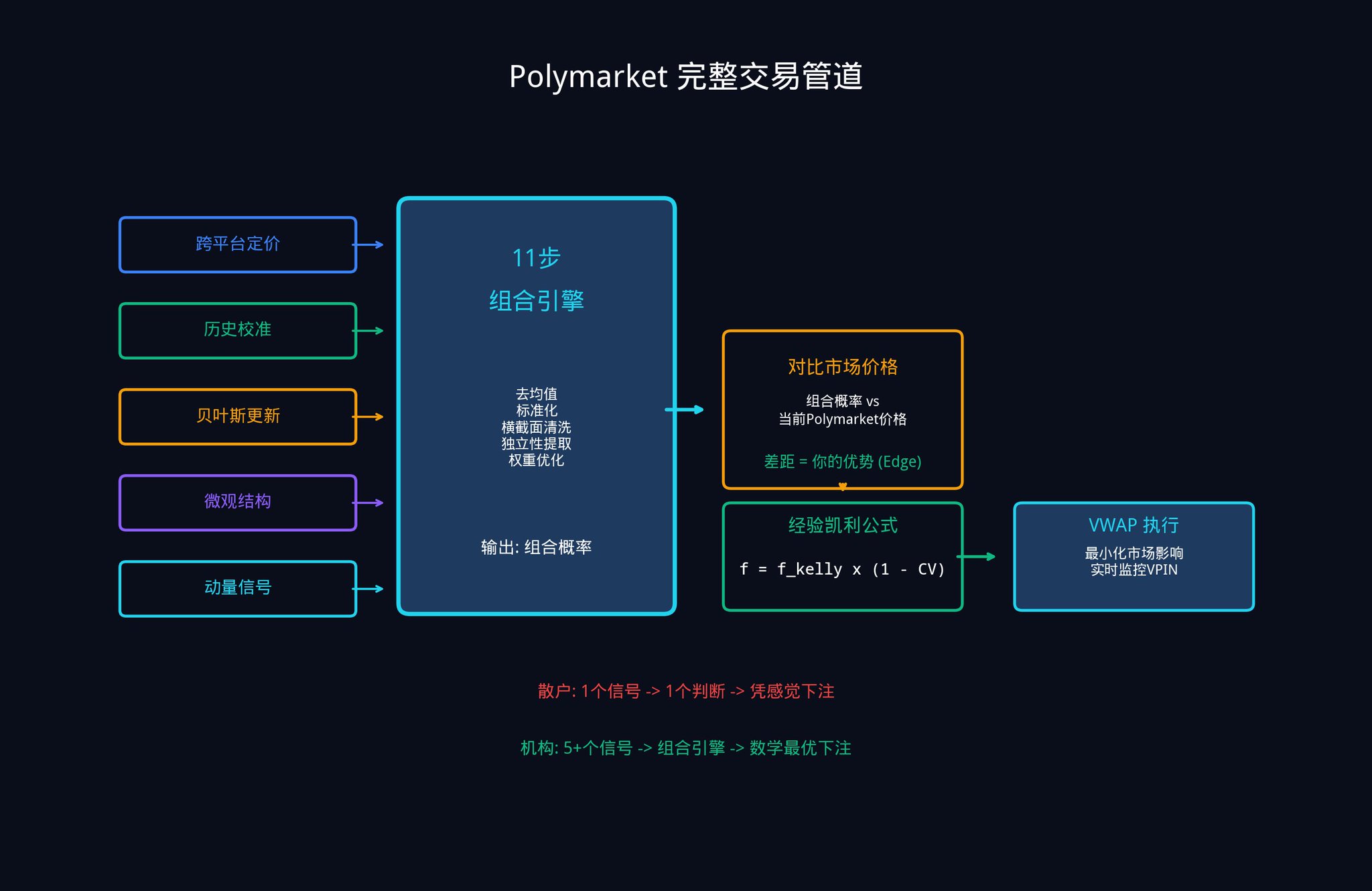
Putting everything together, the complete workflow is as follows:

1. Five or more input signals, each generating an implicit probability estimate

2. Processed through an 11-step combination engine

3. Outputs a single weighted composite probability

4. Compared to the current market price to calculate your Edge

5. Determine bet size using the empirical Kelly formula

6. Optimize execution using VWAP (Volume-Weighted Average Price) to reduce the impact of your large order on the market price

7. Monitor real-time VPIN changes and promptly adjust your strategy when informed traders become active

This framework is particularly valuable for prediction markets for a simple reason: the vast majority of your competitors are trading with a single model, a single data source, and a single probability estimate. But now you know how to combine multiple weak signals into a strong signal. That is your structural advantage.

Advanced Exercise 4:

Choose a Polymarket contract you are interested in. Try to estimate its probability from at least three different angles (e.g., cross-platform pricing, historical calibration, recent news events). Then simply take a weighted average and see if there is a gap between your composite estimate and the current market price. If there is, congratulations, you have just manually completed a simplified version of an Alpha combination.

Recommended reading: Edward Thorp's A Man for All Markets. Thorp is a pioneer in applying the Kelly criterion in the investment field, and this book very simply explains how he made money using mathematics in both the casino and Wall Street.

Part 6: Implementing This System with insiders.bot

At this point, you might be thinking: I understand the logic of this system, but how can I possibly build it from scratch alone?

The good news is, you don't need to start from scratch.

While building insiders.bot (@insidersdotbot), the concept of the "Active Management Law" mentioned in this article, that is, IR = IC x √N (where your overall system performance is equal to the accuracy of a single signal multiplied by the square root of the number of independent signals), gave us a lot of inspiration.

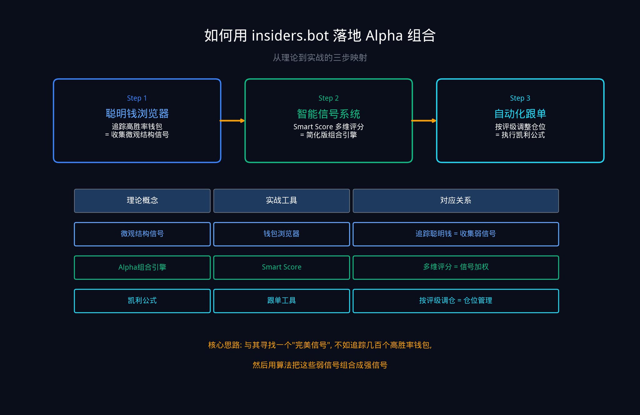
Here are three steps you can take immediately to get started.

Step One: Collect Your Signal Feedstock Using the Smart Money Browser

Open insiders.bot's Smart Money Browser. Through the filter panel, you can find the best-performing wallets on Polymarket based on metrics such as win rate, total P&L, and trading frequency.

Each movement in these wallets is a "microstructural signal" for you (remember the fifth category in the five signal categories discussed in the second part?). While a single wallet's signal may be weak (low IC), when you track dozens of wallets simultaneously, you are creating a "signal combination" as mentioned in the article. This is the core of the Active Management Law: the larger N, the higher the IR.

Step Two: Achieve an Alpha Combination Using the Intelligent Signal System

Our Intelligent Signal System (SIGNALS tab) is essentially a simplified version of an Alpha combination engine. When high-quality wallets make large trades, the system generates signals and, through the Smart Score, integrates historical win rates, total P&L, bet stability, category performance, position size, and other dimensions to provide a strength rating.

LOW: Meets the basic standard but trader advantage is average. Corresponds to a low IC signal, requiring more signals for combination.

MEDIUM: Has a good track record, showing strong conviction. Corresponds to a medium IC signal and can be moderately allocated.

HIGH: Heavy betting from top-performing wallets. Corresponds to a high IC signal, with the combination engine assigning a high weight.

What this scoring system does is essentially the same as the 10th step in the 11-step engine in part three (setting optimal weights, that is, allocating funds based on each signal's independent contribution and stability): assigning different weights to each signal based on a comprehensive evaluation of multiple dimensions.

Step Three: Execute Your Kelly Formula with a Copy Trading Tool

When you receive a HIGH-rated signal, you can use our automated copy trading tool to set proportional or fixed amount copy trading.

Remember the empirical Kelly formula mentioned in Part Five (f_empirical = f_kelly x (1 - CV_edge), which means your bet size should be discounted based on your uncertainty): the more uncertain your estimate, the less you should bet.

For LOW-rated signals, decrease your position size.

For HIGH-rated signals, you can moderately increase your position size. Let math guide your decision-making, not emotions.

Conclusion

Let's return to the initial question.

A single signal is weak. Seeking that perfect signal is completely misguided.

The Fundamental Law of Active Management (IR = IC x √N) mathematically proves: combining many weak independent signals beats finding one strong signal. Your information ratio grows with the square root of the number of truly independent signals you deploy.

The 11-step Alpha Combination Engine provides you with a precise method to calculate optimal weights. These weights reflect the independent contribution of each signal, penalize noise, and eliminate shared variance between signals.

Applied to market prediction, this framework transforms five or more implied probability signals into a single composite estimate. This estimate has been shown to be more accurate than any individual component.

Combine this with the empirical Kelly formula for position management, which correctly aligns your position size with how confident you should actually be, rather than how confident you feel.

Compound the longest-running advantage, built on the most honest model of what you really know.

Finally, I want to leave you with a question:

If an institutional trading desk, combining hundreds of signals, can only achieve an information ratio between 0.05 and 0.15, then what is a system claiming to consistently pick winners with high confidence from a single model really saying?