Original Title: Toward Black-Scholes for Prediction Markets: A Unified Kernel and Market-Maker's Handbook

Original Source: Daedalus Research

Translation, Annotations: MrRyanChi, insiders.bot

On the first day of founding @insidersdotbot, a user asked me if it was possible to provide liquidity through our product. With Polymarket launching a liquidity provision incentive program, discussions about liquidity provision in various groups have become increasingly intense.

However, like arbitrage, liquidity provision is a subject that requires rigorous mathematics to discuss, not just a matter of placing orders on both sides to earn money by providing liquidity. Traditional DeFi market makers have already made a fortune, but market makers in prediction markets are still in the early stages and have a lot of room for profit.

Coincidentally, some time ago, upon a recommendation from a certain quant giant, I came across an academic paper by @0x_Shaw_dalen for @DaedalusRsch, which thoroughly elaborated on the entire Polymarket liquidity provision strategy's logic and how to implement these strategies.

This original article is 100 times more technical than the previous one, so there was a massive amount of rewriting, research, and analysis done to ensure that everyone can understand the full picture of liquidity provision in prediction markets without the need for additional references.

For the previous article, please see "The Polymarket Arbitrage Bible: The Real Gap Lies in Mathematical Infrastructure"

Whether your goal is to become the next major prediction market player or to achieve significant results through airdrops and liquidity incentives, you need to have a thorough understanding of institutional-level liquidity provision techniques, which is exactly what this article can offer you.

Foreword

Before we begin, let me ask you two questions.

First one: You are providing liquidity on Polymarket, and the contract for "Trump Winning the Election" is currently priced at $0.52. You have placed a $0.51 buy order and a $0.53 sell order. Suddenly, CNN reports a major news story. What should your new spread be? $0.02? $0.05? $0.10?

You don't know. Nobody knows. Because there's no formula telling you "how many basis points this news is worth."

Secondly: You are market-making in three markets simultaneously: "Trump wins Pennsylvania," "GOP wins the Senate," "Trump wins Michigan." On election night, the results for the first key state are announced. The three markets experience intense volatility simultaneously. Your entire investment portfolio loses 40% in 3 minutes.

Upon reflection, you realize the issue wasn't a misjudgment of direction, but the fact that you didn't have any tools to measure the magnitude of the risk associated with "the simultaneous movement of these three markets."

These two issues were resolved in the traditional options market in 1973.

In 1973, the Black-Scholes formula provided everyone with a common language. Market makers knew how to price spreads (implied volatility). Traders knew how to hedge the systematic risk of multiple positions (Greeks alphabet and correlations). The entire derivatives ecosystem, from variance swaps and the VIX index to correlation swaps, was built on this foundation.

Had the privilege of witnessing the wisdom of the BS model's inventor earlier at a Chinese university

But in the 2025 prediction market? Market makers adjust spreads based on intuition. Traders assess volatility based on gut feeling. No one can accurately answer, "What is the belief volatility of this market?"

The current prediction market is akin to the options market before 1973.

And this is not just a theoretical issue but a real-world problem, involving real money.

Polymarket now has a comprehensive market maker incentive system [15][16], with over $10M in incentives used by market makers. But here's the problem: if you don't have a pricing model, how do you know how tight the spread should be?

If it's too wide, you won't receive a reward (because others are tighter than you).

If it's too narrow, you'll be front-run by informed traders.

Without a model, you're like a blind man touching an elephant—luck might earn you some rewards, bad luck might make you lose your capital.

It wasn't until I saw Shaw's paper [1] that I realized.

What it did, essentially, was: it essentially wrote a whole set of Black-Scholes for the prediction market. Not just a brand new pricing formula— but an entire suite of market-making infrastructure: from pricing to hedging, from inventory management to derivatives, from calibration to risk management.

As a Polymarket trader, as well as the founder of the @insidersdotbot trading platform, I've had in-depth conversations over the past year with numerous market-making teams, quantitative funds, and trading infrastructure developers. I can tell you: what this paper addresses is exactly the question everyone is asking but no one can answer.

If you don't know what Black-Scholes is, that's okay, this article will explain from scratch, you don't need much basic knowledge of market-making.

If you do know, then you'll be even more excited because you'll realize what this means: implied volatility, Greeks, variance swaps, correlation hedging, all the tools of the traditional options market are about to enter the prediction market.

After reading this article, you will have a complete market-making pricing framework that will upgrade you from "pricing spreads off the top of your head" to "pricing spreads with formulas".

Chapter 1: The First Stop of Volatility Pricing - The Black-Scholes Model

Before discussing the prediction market as an event contract/binary option, we need to first understand one thing: What did Black-Scholes actually do? And why is it so important?

Before 1973: Options = Gambling

Before 1973, options trading was basically like this:

You think Apple stock will rise, you want to buy the right to "buy Apple at $150 in one month" (call option).

Here's the problem: How much is this right worth?

No one knew.

The seller says, "$10." The buyer says, "Too expensive, $5." Finally, it's settled at $7.50.

This was options pricing before 1973— bargaining. There was no formula, no model, no concept of the "correct price." Everyone was guessing.

The essence of an option is: to buy a if I guess right opportunity with a small amount of money.

The Core Insight of Black-Scholes

In 1973, Fischer Black and Myron Scholes published a paper [2], proposing what seemed like a simple idea:

The price of an option depends only on one thing you do not know—volatility.

It does not depend on whether the stock will go up or down (direction). It does not depend on how much you think it will go up (expected return). It only depends on how much it will fluctuate.

Why? Because they proved one thing: If you hold an option, you can "replicate" the returns of this option by continually buying and selling the underlying stock. The cost of this replication process depends only on volatility.

We can understand this with middle school math:

Imagine you are playing a coin game. Heads earn $1, tails lose $1. Someone sells you an "insurance": If the final result is a loss, the insurance company will cover you. How much is this insurance worth?

The key is not whether the coin is "fair" (whether the probability of heads is 50%). The key is how large the fluctuation is for each flip.

If each flip is ±$1, the insurance is cheap. If each flip is ±$100, the insurance is very expensive.

Greater volatility → more expensive insurance → more expensive option. It's that simple.

What Black-Scholes did was to turn this intuition into a precise formula.

Why Did This Change the Market-Making Model?

Before Black-Scholes: Options were gambling. Traders priced based on intuition, lacking a common language.

Black-Scholes established a whole consensus for options:

A common language was born. Everyone started using "implied volatility" to quote. You no longer say "this option is worth $7.50," you say "the implied volatility of this option is 25%." It was as if everyone suddenly started speaking the same language.

Risk has been decomposed. The risk of options has been broken down into several separate "dimensions" — Delta (directional risk), Gamma (acceleration risk), Vega (volatility risk), Theta (time decay). These are called Greeks. Market makers can precisely hedge the risk of each dimension.

A new layer of derivatives emerged. With a common language, you can build new products on top of it. Variance swap (betting on volatility magnitude), correlation swap (betting on the correlation between two assets), VIX index ("fear index") — all of these are the "offspring" of Black-Scholes.

The CBOE was established. The Chicago Board Options Exchange was founded in 1973 — the same year as the Black-Scholes paper. This is not a coincidence. With a pricing formula, options could be traded standardizedly [3].

In other words, Black-Scholes transformed options from "gambling" to "financial engineering." It is not just a formula — it is the starting point of a whole infrastructure.

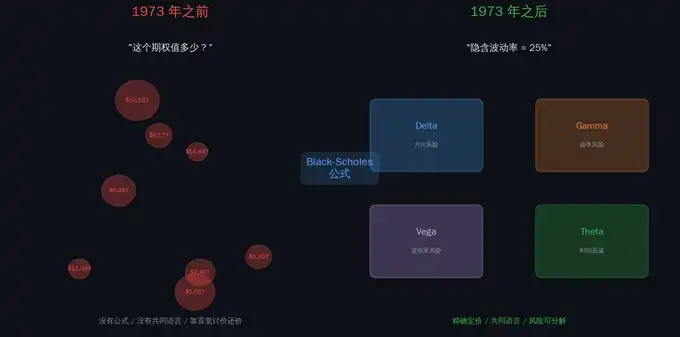
Comparison around 1973

Now, prediction market making is akin to pre-1973

In 2025, the monthly trading volume in prediction markets exceeded $13 billion [9]. NYSE's parent company ICE invested $2 billion in Polymarket, valuing it at $8 billion [7]. Kalshi and Polymarket collectively hold 97.5% of the market share.

However —

How do market makers price spreads? By intuition.

How do traders determine if a contract's volatility is "expensive" or "cheap"? By feel.

How do you hedge the correlation between two related markets? No standard tools.

When a news shock hits, how should spreads be adjusted? Everyone has their own ad hoc methods.

This is the pre-1973 options market.

And the job of the model in this article is: to write a Black-Scholes for the prediction market's liquidity provider.

Chapter 2: Logit Transformation - Making the BS Model Fit Prediction Markets

First Question: What Is the Difference Between Prediction Markets and Stock Markets?

In theory, stock prices can go from $0 to infinity. Apple's price can go from $150 to $1500, or it can drop to $0.

On the other hand, prediction market contract prices always range between $0 and $1.

The price of a YES contract for "Trump Winning the Election" reflects the market's belief in the likelihood of this event. $0.60 means the market believes there is a 60% chance of it happening.

This difference may seem subtle, but it poses a significant mathematical problem:

You cannot directly apply Black-Scholes.

Why? Because Black-Scholes assumes prices can freely move along the entire real number line (technically, the positive half-line). However, probabilities are "bounded" between 0 and 1. As probabilities approach 0 or 1, their behavior becomes very peculiar — the changes become slower and stickier near the boundaries.

For example, imagine running in a corridor. In the middle of the corridor, you can run freely. But as you get closer to the walls, you must slow down, or you'll hit the wall. Probabilities behave similarly — the closer they are to 0 or 1, the harder it is to "move." Going from $0.50 to $0.55 is easy (just a piece of news), but going from $0.95 to $1.00 is extremely difficult (requires nearly certain evidence).

Solution: Logit Transformation - Turning the Corridor into a Playground

The first key step of the paper: Do not model the probability p directly; instead, model its logit transformation.

What is the logit?

x = log(p / (1-p))

It transforms the probability p into "log odds." Let's look at a few examples:

· p = 0.50 (even odds) → x = log(1) = 0

· p = 0.80 (highly likely) → x = log(4) = 1.39

· p = 0.95 (almost certain) → x = log(19) = 2.94

· p = 0.99 (extremely certain) → x = log(99) = 4.60

· p = 0.01 (almost impossible) → x = -4.60

A probability range from 0 to 1 is mapped to the entire real number line from -∞ to +∞.

The corridor becomes the playground. The "stickiness" of probability near 0 and 1 disappears. Now, you can freely apply all traditional mathematical tools on x.

You may have encountered the Logit transformation: it is the inverse of the sigmoid function in machine learning. The sigmoid function compresses any number to between 0 and 1 (used for probability prediction). The logit does the opposite: it "expands" probabilities between 0 and 1 to the entire real number line.

Why do this? Because the behavior of probabilities near 0 and 1 is quite "twisted" — going from 0.95 to 0.96 and from 0.50 to 0.51, even though both increase by 0.01, the information content is completely different. The logit transformation flattens this "unevenness." In logit space, equally spaced changes represent equal amounts of informational impact.

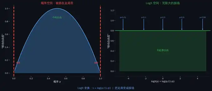
Logit Transformation

Jumps, Diffusion, and Drift: Belief Diffusion with Jumps

Now we are in logit space. Next, the paper presents the core rate of change model as follows:

dx = μ dt + σ_b dW + Jump Term

Don't be intimidated by the formula. Three parts, each should become your intuition in market-making:

Diffusion (σ_b dW): This is belief volatility. The speed at which probabilities slowly change due to continuous information flow (poll updates, analyst comments, social media sentiment) in the absence of significant news. This is the "implied volatility" of prediction markets — the central concept of the entire article. Market maker spread, derivative pricing, risk management — all revolve around this σ_b.

Jump: A probability spike caused by breaking news. Key missteps in a debate, unexpected policy announcements, sudden withdrawals — these are not "slow diffusion" but "instantaneous jumps".

Drift (μ): The time-dependent probability's "natural trend". But there's a catch — drift isn't free, it's fully locked in. Here's why.

Imagine you're watching an election poll.

Most of the time, the support rate fluctuates by 0.1-0.3 percentage points a day — this is diffusion (σ_b dW). Like ripples on the water's surface, continuous but gentle.

Then one night, a candidate says a disastrous remark in a debate. Overnight, the support rate drops from 55% to 42% — this is a jump. Like a stone thrown into water.

This model captures both the "ripples" and the "stone". The traditional Black-Scholes only has ripples (pure diffusion), without the stone (jump). This paper's model is more comprehensive — because predicting market news shocks is far more frequent and severe than in the stock market.

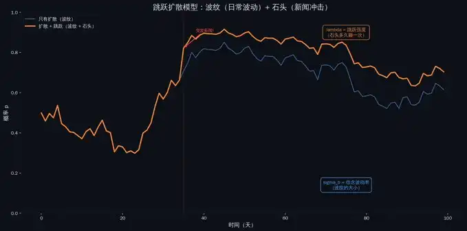
Jump-Diffusion Model

Locked-In Drift: Market Maker's True Alpha

This is one of the most exquisite parts of the entire paper.

In traditional Black-Scholes, there's a famous conclusion: Option pricing doesn't need to know if a stock will rise or fall. You don't need to predict if Apple will rise or fall next year to price an Apple option. Because drift in the risk-neutral measure gets "replaced" by the risk-free rate.

Similar things happen in predictive markets: probability p must be a martingale. In the absence of new information, your best guess about the probability is the current probability. If the market believes Trump has a 60% chance of winning, then in the absence of new information, tomorrow's best guess is still 60%.

This means: Drift μ is fully locked in. Once you know the belief volatility σ_b and jump behavior, drift is automatically set. You don't need to guess the specific number for drift.

For market makers, this is great news. You don't need to predict "Will Trump win" (direction); you just need to estimate "How uncertain the market is" (volatility). Direction is something everyone is guessing at—you have no edge there. But volatility is something that can be precisely estimated from data—that's your edge.

In simple terms, you don't need to know if it will rain tomorrow (direction); you just need to know how uncertain the weather forecast is (volatility). You price for "uncertainty," not for "direction." That's the fundamental difference between market makers and retail traders.

Three Tradable Risk Factors

After Drift is hedged, what's left? Market makers need to focus on these three factors:

Belief Volatility σ_b: The "daily speed of randomness" in the probability in the absence of major news. This is the core input for your pricing spread. σ_b high → spread widens. σ_b low → spread narrows.

Jump Intensity λ and Jump Size: How often does unexpected news arrive? How much does the price jump each time? This determines how much "insurance" you need (this is what derivatives in Chapter Four do).

Cross-Event Correlation and Common Jumps: Will two correlated markets move simultaneously due to the same news? This determines your portfolio risk.

These three factors are the "dashboard" for predicting market makers. Just as traditional options market makers stare at the implied volatility surface every day, future predictive market makers will watch σ_b, λ, ρ.

Chapter Three: Market Maker Playbook

The theory holds. But what market makers care about is: How does this thing make money?

Predictive Market Greeks

In the traditional options market, Greeks (Greek letters) are the lifeblood of market makers. Delta tells you how much directional risk there is, Gamma tells you acceleration risk, Vega tells you the impact of volatility changes.

This paper defines a complete set of Greeks for predictive markets [1]:

Most important is Delta, Delta = p(1-p)

This is Directional Sensitivity — how much does the probability p change when x changes by 1 unit in logit space.

Pay attention to this formula: p(1-p). This thing will appear repeatedly — it's the "universal factor" of the whole article.

When p = 0.50, Delta Max = 0.25. When p = 0.95, Delta = 0.0475. When p = 0.99, Delta = 0.0099.

How do market makers use this? Near p = 0.50, the same information shock will cause the largest price movement — you need a wider spread to protect yourself. Near p = 0.99, even though a large change occurs in logit space, the price hardly moves — you can quote a very narrow spread.

For example, an election is currently 50-50. A news piece comes out, the probability may jump from 50% to 55% — a 5 percentage point change. But if it's currently 99-1, the same news may only move the probability from 99% to 99.2% — hardly a change. The closer to a certain outcome, the harder it is to shake.

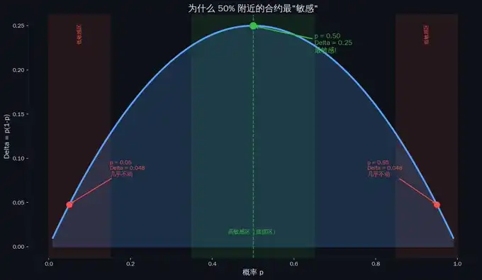
Delta Sensitivity

The other three important factors are Gamma, Belief Vega, and Correlation Vega.

Gamma = p(1-p)(1-2p): This is the "news nonlinearity". When the probability is not at 50%, the impact of good news and bad news is asymmetric. If p = 0.70, the impact of good news is smaller than bad news (because it's already high, with limited upside). Market makers need to know this because asymmetry means your inventory risk is also asymmetric.

Belief Vega: How sensitive is your position to changes in belief volatility? If σ_b suddenly increases (for example, the day before a debate), how will your position value change?

Correlation Vega: If you hold positions in two correlated markets, how will changes in their correlation affect you?

Four Types of Risk

The paper categorizes all risks facing market makers into four main types [1]:

Directional Risk (Delta): Which way is the probability moving? This is the most basic.

Curvature Risk (Gamma): Big news hit, is the price reaction asymmetric?

Information Intensity Risk (Belief Vega): Is the "uncertainty" of the market itself changing? For example, uncertainty skyrocketing before a debate.

Cross-Event Risk (Correlation Vega + Joint Jump): Will your multiple positions lose money simultaneously due to the same news?

For example, if you are an insurance company, Directional Risk is "Will this house catch on fire?" Curvature Risk is "If it catches on fire, will the loss be linear or exponential?" Information Intensity Risk is "Is this year particularly dry, is the probability of fires increasing?" Cross-Event Risk is "If one house catches on fire, will the house next door also catch on fire?"

A stellar market maker will manage these four types of risk separately, rather than blending them together.

Inventory Management: How much inventory you have and how to adjust prices

The core daily issue for a market maker is: How much inventory do I have, and how should I adjust the spread?

The paper moves the classic Avellaneda-Stoikov market-making model [6] to logit space:

Reserve Quote = Current logit value - Inventory × Risk Aversion × Belief Variance × Remaining Time

Total Spread ≈ Risk Aversion × Belief Variance × Remaining Time + Liquidity Premium

No need to memorize the formulas. Just remember three rules:

More Inventory → More Skewed Quote. If you have too many YES contracts on hand, you will lower the selling price of YES (encouraging others to buy) and push the buying price of YES even lower (not wanting to buy more). This is the market maker's "self-preservation" — controlling inventory through price adjustments.

Higher Volatility → Wider Spread. The more uncertain the market, the greater the risk you take on, and the more compensation (spread) you demand. On Debate Night when σ_b spikes, your spread should automatically widen.

Closer to Expiry → Narrower Spread. Because remaining uncertainty is diminishing. On Election Day morning when the outcome is nearly certain, the spread should be very narrow.

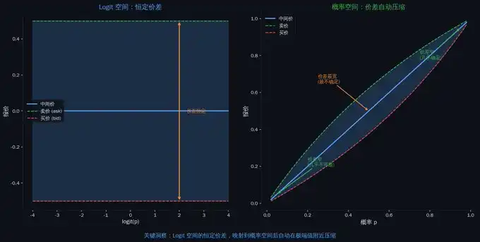
But here's the twist: When you map a quote in logit space back to probability space, the spread automatically compresses near extreme probabilities. This is because Delta = p(1-p), and around p ≈ 0 or p ≈ 1, a unit change in logit space corresponds to a small change in probability space. So even if you maintain a constant spread in logit space, when mapped back, the spread near extreme prices automatically narrows.

This aligns perfectly with Polymarket's incentive mechanism: Near extreme probabilities, you can quote a very narrow spread (due to low risk), receive a higher Q-score, earn more liquidity rewards. The model automatically achieves this for you.

For example, suppose you are a used car dealer. If the market price of a car is very uncertain (could be worth $10,000 or $20,000), you would offer a wide spread—Buy at $12,000, Sell at $18,000. If the market price is certain (around $15,000), you would offer a narrow spread—Buy at $14,500, Sell at $15,500. Market makers do the same thing. They just "sell" probability contracts instead of used cars.

Market Maker Spread Mechanism

Chapter Four: The Market Maker's Vault - Five Risk Tools You'll Eventually Need

The first three chapters gave you tools to price spreads and manage inventory. But a core contradiction faced by market makers has not been resolved yet:

You earn the spread (steady small gains each day), but you take on tail risk (occasional large losses).

On Debate Night, volatility spikes 5x, wiping out a month's profit overnight. On Election Night, three markets crash simultaneously, and the portfolio loses 40%. Probability suddenly jumps from $0.60 to $0.90, causing a massive loss on your NO inventory.

In the traditional options market, market makers use derivatives to hedge these risks. Variance swaps hedge volatility spikes. Correlation swaps hedge multi-market correlations. Barrier options hedge extreme prices.

The prediction market currently lacks these tools. But this paper provides a complete mathematical foundation, where each product's pricing formula directly comes from the second chapter's logit space model.

What's the relationship between these products and the earlier framework? Quite simple: the model in the second chapter gives you three risk factors (σ_b, λ, ρ), the Greeks in the third chapter tell you how sensitive your position is to these factors, the derivatives in the fourth chapter allow you to precisely hedge the risk of each factor. Without derivatives, you know you have risk but can't eliminate it. With derivatives, you can "sell" unwanted risk to willing counterparties.

This is also why derivatives are not just "toys for sophisticated players." They are key to whether a market maker can survive long term. Without hedging tools, a market maker can only widen spreads to protect themselves. Wider spreads mean poorer liquidity. Poorer liquidity means the market cannot grow.

Derivatives → Hedging → Tighter Spreads → Better Liquidity → Larger Market.

This positive cycle occurred in the options market in 1973. Now it's the prediction market's turn.

This section will mention five products, each addressing a specific market-making pain point, each designed as a function a prediction market maker/tool could perform. (So, if there's demand, maybe one day @insidersdotbot will create them. Stay tuned. If you want to develop these products yourselves, we're also happy to provide our trading API and data API.)

Product One: Belief Variance Swap - Volatility Insurance

What problem does it solve? You're market-making in five markets, earning a steady $200 spread income per day. Then debate night arrives, and volatility skyrockets fivefold, causing you to lose $3,000 overnight. Half a month's profit gone.

You earn the spread (stable small money), but you bear volatility risk (unstable large money). These two are mismatched.

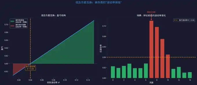
How does it work? You and the counterparty agree on an "execution volatility." If the actual volatility is higher than this level, the counterparty reimburses you; if it's lower, you reimburse the counterparty. Essentially, it's volatility insurance.

Specific Example: For example, two weeks before the election, you buy a belief variance swap, agreeing to execute at a volatility of σ² = 0.04. On debate night, volatility spikes to 0.10, and you receive a payout of 0.06, covering stock losses. If the debate is boring and volatility is only 0.02, you lose 0.02—this is the premium.

What is it priced off of? Fair execution price = Variance of daily volatility + Variance of news jumps. The two parts come from σb (diffusion) and λ (jumps) of the model in Chapter 2.

Analogy in Traditional Markets: The VIX index is the price of a basket of variance swaps [14]. It tells you "what the market thinks the volatility will be for the next 30 days." The global variance swap market has reached trillions of dollars [10].

Can You Use It Now? Currently, no platform offers this product. But if you are a developer, the appendix of the paper has the complete pricing formula. If you are a market maker, you can start with a simplified version: reduce inventory in high volatility periods, increase inventory in low volatility periods, essentially manually doing a variance swap.

Belief Variance Swap

Product Two: p(1-p) Curve - Predicting the "Fear Index" of the Market

What Problem Does It Solve? You want to know "how tense the market is right now," but there is no standardized indicator.

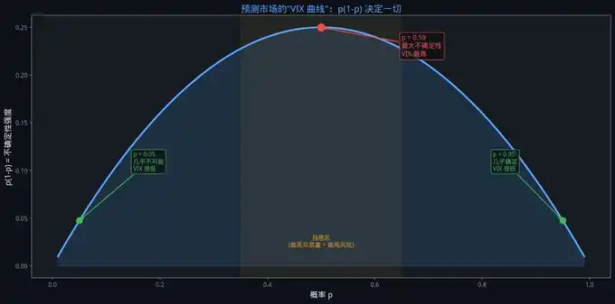
How to Achieve It? Remember the Delta = p(1-p) from Chapter 3? This formula is not just a Greek—it is also an "uncertainty thermometer."

When p = 0.50, p(1-p) = 0.25—maximum uncertainty. When p = 0.90, p(1-p) = 0.09—uncertainty has decreased almost threefold.

When p = 0.99, p(1-p) = 0.0099—almost no uncertainty left.

Why Is This Useful? When you see a contract go from $0.50 to $0.60, and p(1-p) goes from 0.25 to 0.24, the uncertainty hardly changes, and the spread does not need adjusting. But if it goes from $0.80 to $0.90, and p(1-p) goes from 0.16 to 0.09—uncertainty decreases by almost half, allowing you to tighten the spread and earn more liquidity rewards. Even with the same $0.10 increase, the market-making strategy should be completely different.

Benchmarking in the Traditional Market: p(1-p) also has similarities with the VIX index [14]. The VIX tells you "how fearful the market is." p(1-p) tells you "how uncertain the market is."

Available Now! The p(1-p) curve is the only one among the five products that can be used immediately today. One line of code: uncertainty = p * (1 - p). Add it to your market-making strategy, and you can dynamically adjust the spread based on uncertainty.

VIX Curve

Product Three: Correlation Swap - Election Night Earthquake Insurance

What Problem Does It Solve?

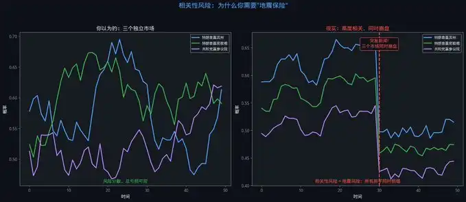
You are market-making in three markets: "Trump Wins Pennsylvania" ($5,000 in stock), "Trump Wins Michigan" ($5,000 in stock), "Republicans Win Senate" ($3,000 in stock). If these three markets were independent, losing money in one might be offset by profits in the others. However, in reality, they are highly correlated—a piece of news can cause all three markets to crash simultaneously. You are not losing just $5,000—you could be losing $13,000.

How Does It Work? You and the counterparty agree on an "execution correlation." If the actual correlation exceeds this level, you receive a payout. During the 2008 financial crisis, the correlation of all assets suddenly spiked to nearly 1—those holding correlation swaps made a fortune, while those without were annihilated.

What Is It Priced On? The model in Chapter Two has a "common jump" parameter—multiple markets jump simultaneously due to the same news. The pricing of a correlation swap directly depends on this parameter. Without a model to estimate the "strength of common jumps," you cannot price this insurance.

What Can You Do Now? Currently, there are no formal correlation swap products. However, you can approximate using a simple method: take opposing positions in highly correlated markets. For example, if you hold YES stock in "Trump Wins Pennsylvania," you can also hold YES stock in "Trump Wins Michigan"—you can actively reduce inventory in one market to lower correlation exposure. Mathematically, this model is not perfect, but it is much better than being unhedged.

Relevance Risk

Product Four: Corridor Variance - Precise Insurance for the "Swing Region"

What Problem Does It Solve? You bought a variance swap covering the entire probability range, but you realize that when the probability is above 0.90, the volatility is very low, and you are paying insurance premiums for the low-risk range unnecessarily. What you really need to protect is the "swing region" from 0.35 to 0.65 — where the order flow is the highest, information toxicity is the greatest, and it is most vulnerable to front-running by informed traders.

How Is It Achieved? Corridor variance only accumulates variance when the probability is within a certain range. You can purchase insurance only for the "swing region" and not pay for the calm region.

What Is It Priced On? Corridor variance requires knowledge of the local volatility in different probability ranges. This information comes directly from Chapter Five's belief volatility surface — the surface tells you "around p = 0.50, what is the volatility; around p = 0.90, what is the volatility." Without the surface, you cannot price corridor variance.

Real-World Scenario: You are a market maker mainly active in the "swing region" (0.40-0.60). You purchase a corridor variance contract that only covers this range. When the probability experiences sharp fluctuations within this range, you receive a payout. When the probability reaches above 0.85 in the "safe zone," corridor variance stops accumulating — you do not have to pay insurance premiums for that range. Lower premium, more precise coverage.

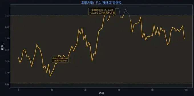
Corridor Variance

Product Five: First Touch Note - Stop-Loss Insurance for Extreme Prices

What Problem Does It Solve? You are a market maker, and "Trump Wins" is currently at $0.60. You hold some NO inventory. If the probability suddenly surges to $0.90, your NO inventory faces significant losses. You can set a stop-loss order, but in prediction markets, stop-loss orders are often "run over" (price briefly touches your stop-loss price and then retraces, forcing you to liquidate, and then you helplessly watch the price return to its original position).

How Is It Achieved? "If the probability breaks $0.80 before election day, pay me $1." This is stop-loss insurance for extreme prices — no need to set a stop-loss manually, instead hedge precisely using a financial contract.

What Does Pricing Depend On? Pricing a First Touch Option requires knowing the probability path of "touching a certain level." This is a classic first-passage-time problem that directly depends on the parameters σ_b and λ from Chapter 2. The more frequent the jumps (larger λ), the higher the probability of reaching an extreme level, making the option more expensive.

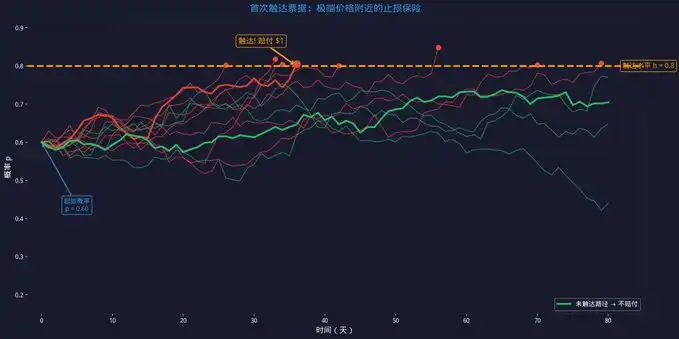
First Touch Option

Interconnected Five Major Products

The five products mentioned in this section are not isolated. They form a complete market maker risk management toolbox:

· Variance Swap hedges overall volatility risk.

· Corridor Variance precisely hedges risk within a specific range.

· Correlation Swap hedges multi-market linkage risk.

· First Touch Option hedges extreme price risk.

The p(1-p) curve provides a common "uncertainty" language for everyone.

And the pricing of all these products goes back to the same place: the logit space jump-diffusion model from Chapter 2. σ_b prices Variance Swaps and Corridor Variance. λ prices First Touch Options. The common jump parameter prices Correlation Swaps.

This is why this paper is not just "one model" — it is the starting point for a whole market infrastructure.

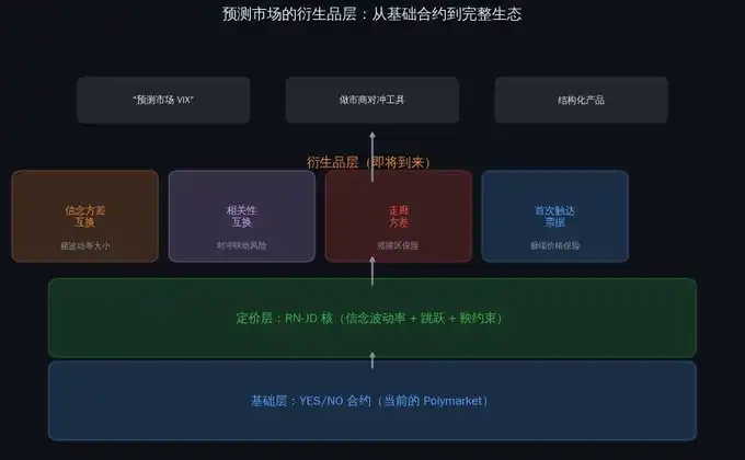
Derivatives Layer Overview

These products mentioned in this section (except p(1-p)) do not yet exist on any prediction market platform. The closest entry is Polymarket's CLOB API [15] — you can build automated market-making strategies on it, using the paper's Greeks to manage inventory. Of course, when @insidersdotbot opens its API, we also welcome everyone to contact us at any time.

As the saying goes, Polymarket's development has a long way to go and requires everyone to work together to build it.

If you are a developer, the paper's appendix contains the complete pricing formula.

If you are a liquidity provider, you can start by optimizing your existing spread strategy using p(1-p) and σ_b — this can be done immediately through a simple script without waiting for the derivatives market to be established.

Chapter Five: Data Calibration - Extracting Signals from Noisy Data

No matter how beautiful a theoretical model is, if parameters cannot be calibrated from real data, it is worthless.

The original paper dedicated a lot of space to discussing the calibration pipeline [1], which is also the key difference between it and purely theoretical papers — an effective, reliable, and actionable conclusion.

What is "Calibration"?

Imagine you buy a thermometer. Its scale is printed, but how do you know if it's accurate? You need to put it in ice water (should read 0°C) and boiling water (should read 100°C), and then adjust it. This process is calibration.

Our model is similar. The earlier chapters defined a beautiful mathematical framework, but to implement it, there are several key parameters in the framework that need to be extracted from real data:

σ_b: Belief volatility. How much does the probability "naturally fluctuate" each day?

λ: Jump intensity. How often do sudden news events occur?

Jump size distribution: How large are the jumps each time?

η: Microstructure noise. How many "fake signals" are in the market price?

These parameters are not arbitrarily chosen. They must be extracted from real market data. Calibration is a critical step in transitioning the model from "theoretically correct" to "practically applicable in the field."

Issue: The Price You See Is Not the True Probability

Opening Polymarket, you see the latest trade price for "Trump Winning Election" is $0.52.

Is this $0.52 the "true market belief"? No. It is filled with three main types of noise:

Spread Noise: The "latest trade price" you see may just be someone market-buying into a resting limit order. If the bid is $0.51 and the ask is $0.53, the "true belief" may be around $0.52. However, the latest trade price could be $0.51 or $0.53.

Liquidity Depth Noise: A $500 market order can move the price by 3%. This is not a "shift in market belief" but rather "lack of depth in the order book."

Microstructure Noise: High-frequency trading, market maker quote adjustments, network latency—all add noise on top of the true signal.

Observational Model in Papers: Observed logit = True logit + Microstructure Noise. Your task is to recover the true signal from noisy data.

Step One: Kalman Filtering - Signal Recovery from Noise

The Kalman filter is a classic signal processing tool [13]. It was initially developed for the Apollo Lunar Landing program—to track the spacecraft's true position from noisy radar signals.

Core Idea: You have two imperfect sources of information. The Kalman filter finds the optimal weighting between the two.

Source One: Model Prediction. Your jump-diffusion model says, "Based on yesterday's probability and parameters, today's probability should be around X." But the model is imperfect—it doesn't know if there will be news today.

Source Two: Actual Observation. The latest trade price in the market tells you, "The price right now is Y," but the observation is imperfect—it contains noise.

Approach of the Kalman Filter:

Good market liquidity (narrow spread, deep depth) → Small observation noise → Trust observation more.

Poor market liquidity (wide spread, shallow depth) → Large observation noise → Trust model prediction more.

This allocation of "trust" is automatic and optimal. You do not need to manually tune parameters.

This is like driving a car where the GPS tells you "You are on Road A" (observation), but your speedometer and steering wheel tell you "You should be on Road B" (model prediction). Trust the GPS when the signal is strong, and trust the speedometer when the signal is weak (e.g., in a tunnel). The Kalman Filter is a system that does this "automatic trust-switching."

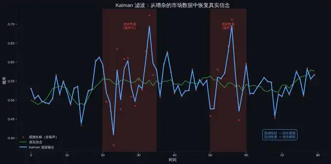
Kalman Filter

Step 2: EM Algorithm - Separating "Daily Volatility" from "News Shocks"

After recovering the true signal, the next question is: which price movements are "normal volatility" (diffusion) and which are "news shocks" (jumps)?

Why separate them? Because the nature of these two types of movements is completely different. Diffusion is continuous and predictable—the volatility today is 2%, it will likely be around 2% tomorrow. Jumps are sudden and unpredictable—one moment it's calm, the next moment there's a 10-point jump in probability.

If you estimate both types of movements together, you will overestimate the daily volatility (because jumps are included), leading to too wide of a bid-ask spread, which means no profit.

How does the EM algorithm separate them?

Imagine you have a pile of balls in front of you, some are red (jumps), some are blue (diffusion), but the lighting is dim, and you can't see the colors clearly.

E Step: For each ball, guess the probability of it being red or blue based on its size. Larger balls are more likely to be red (jumps are usually larger).

M Step: Based on your guesses, calculate the "average size of red balls" (jump parameter) and the "average size of blue balls" (diffusion parameter).

Then repeat: Guess the colors again with the new parameters → Recalculate the parameters with the new colors → Repeat until convergence.

Key constraint: After each M step, recalculate the risk-neutral drift to ensure that the probability remains a martingale. This is the "foundation" of the whole framework—no matter how you separate diffusion and jumps, the martingale property cannot be violated.

The EM algorithm is like listening to an audio recording. The recording has two types of sounds: background music (diffusion) and occasional fireworks (jumps). You want to measure how loud the background music is and how loud the fireworks are separately. If you don't separate them and just measure the total volume, you will get an "average volume"—too high for the background music and too low for the fireworks. The EM algorithm's approach is: first, guess which moments are fireworks and which are background music, then measure them separately. After several rounds, you will be able to accurately separate the two types of sounds.

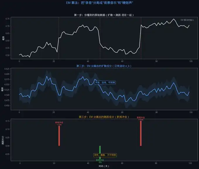
EM Algorithm

Step Three: Build Belief Volatility Surface

After separating diffusion and jump components, you can build a belief volatility surface.

In the traditional options market, implied volatility is not a fixed number. It depends on two dimensions:

· First, time to maturity (more uncertainty as time goes by)

· Second, current price level (different price ranges have different volatilities)

Mapping these two dimensions into a surface gives you a volatility surface [12].

For a market maker, the first thing every morning is to look at the volatility surface — it tells you "what the market thinks future volatility will be like".

Now, market-making predictors can also have their own surface.

What can this surface tell you?

· If the surface suddenly steepens at a certain time (e.g., the day before a debate), it means the market expects high volatility at that time. Market makers should widen spreads in advance.

· If the surface is much higher around p = 0.50 compared to p = 0.80, it means the volatility in the "swing area" is much higher than the "certainty area". You can quote narrower spreads in the certainty area and receive more liquidity rewards.

· If the volatility surfaces of two markets have a similar shape, it means they may be driven by the same factors. You need to pay attention to correlation risk.

In simple terms, the volatility surface is a "heat map" of a weather forecast. The horizontal axis is future dates, the vertical axis is different regions, and colors represent temperature. You can instantly see that "North China will be particularly hot next Wednesday". The belief volatility surface is the "volatility heat map" of the prediction market. The horizontal axis is time to settlement, the vertical axis is the probability level, and colors represent volatility. You can instantly see that "the volatility is highest the day before a debate near a 50% probability".

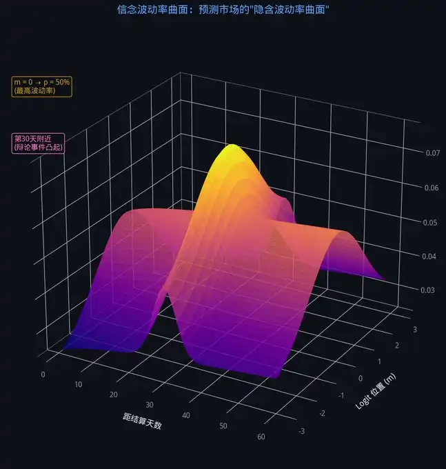
Belief Volatility Surface

Chapter 6: Experiment - Does This Framework Really Work?

Over the first five chapters, we have built a complete framework. In this chapter, we aim to answer the most crucial question: is it really better than existing methods?

How to Evaluate?

The paper used two core metrics [1]:

· Mean Squared Error: It calculates the square of the difference between the predicted value and the actual value at each time point, then takes the average. Squaring significantly penalizes large deviations — the penalty for a deviation of 0.10 is 100 times that of a deviation of 0.01. This answers the question: Does the model occasionally make significant errors?

· Mean Absolute Error: It takes the absolute value of the deviation and then averages them. In simpler terms: what is the average deviation each time?

A good model should have both metrics low — indicating it neither makes occasional significant errors nor consistently makes small errors.

Another crucial point: The model can only use data up to each time point and cannot peek into the future.

Four Opponents

To demonstrate the effectiveness of the above framework, the original paper's model was compared head-to-head with four existing market-making methods.

· Random Walk: Assumes the volatility remains constant. Whether it's a heated debate night or a calm period, the volatility stays the same. It's like a weather forecaster saying "tomorrow will be 25°C" every day — occasionally correct in spring, but way off in winter and summer. The simplest baseline.

· Constant Volatility Diffusion: Similar to random walk, but the volatility is fitted from the data — the "optimal constant." It's like that forecaster changing to "reporting the yearly average temperature every day" — the average error decreases, but it still misses extreme weather.

· Wright-Fisher / Jacobi Model: Models directly in the probability space (between 0 and 1) without a logit transformation. It sounds more "natural" — probabilities are originally between 0 and 1, so why transform them? However, this is a pitfall. When probabilities are close to 0 or 1, small errors in the probability space are exponentially amplified when mapped to the logit space.

· GARCH: The most commonly used volatility model in traditional finance. The core idea is "large volatility is followed by large volatility." It works very well in the stock market. However, in the prediction market, it has two fatal flaws: it does not distinguish between daily volatility and news jumps, and it lacks a martingale constraint.

Result: Total Domination

The market-making model we constructed is optimal in both mean squared error and mean absolute metrics [1].

In terms of mean squared error in logit space, the model used in this paper outperforms the best adversary (constant volatility diffusion) by over an order of magnitude. It outperforms Wright-Fisher and GARCH by 15 to 17 orders of magnitude.

It's not "slightly better." It's "not even in the same league."

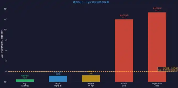
Model Comparison

Why Such a Large Gap?

Martingale constraints eliminate systematic bias. Other models lack this constraint, potentially implying assumptions like "probabilities should move up" or "move down." The martingale constraint in the paper's model ensures the scale is balanced.

Separation of Jumps and Diffusion. The volatility during calm periods is not contaminated by news jumps. GARCH cannot achieve this—it sees a large fluctuation and assumes more will follow, but in reality, calm may return immediately after a jump.

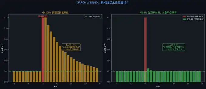
GARCH vs RN-JD

Calendar awareness. The model knows "there's a debate next week" or "next month is election day." Around these known news windows, it automatically increases jump intensity predictions. Other models completely ignore this public information.

The Most Critical Discovery: Modeling in Probability Space is a Dead End

The most shocking finding in the experiment: Directly modeling in probability space catastrophically fails.

Wright-Fisher and GARCH, when mapped to logit space, see mean squared error inflate by 15 to 19 orders of magnitude.

If you are a market maker and you use these models to price spreads, your spread will be completely wrong near extreme probabilities. It's not a 10% bias—it's a bias of 10 to the power of 17. Arbitrageurs will eat you alive within seconds.

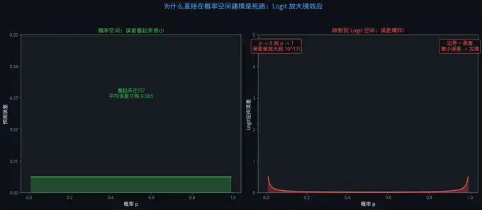
Probability Space Modeling Is a Dead End

This discovery locked in one conclusion: Quantitative modeling of prediction markets must be done in logit space. If you are currently using any method that directly models in probability space (including simple moving averages, linear regression, etc.), first perform a logit transformation before analysis. One line of code (x = log(p/(1-p))), but it can avoid catastrophic errors.

Epilogue: The Market Maker Life from Scratch

Finished reading the six chapters. From the 1973 BS formula, to logit transformation, to Greeks and inventory management, to derivatives, to calibration, to experimental validation.

Now the question is: What's next?

If you are a retail trader — you don't need to implement the entire model. But there are two things worth using immediately:

· First, assess your position risk using p(1-p). If you hold a $0.50 contract, p(1-p) = 0.25, your position is very sensitive to news. If you hold a $0.90 contract, p(1-p) = 0.09, the sensitivity is almost 3 times lower. Same $1,000 position, but the risk is completely different.

· Second, remember "Volatility Matters More Than Direction." When you see a contract price fluctuating dramatically around $0.50, it's not just "market uncertainty" — it's high conviction volatility, meaning high risk. Understanding this difference is more useful than predicting "Will Trump win?"

If you are a market maker — this paper has given you a complete upgrade path:

· Doable Today: Move your analysis from probability space to logit space (x = log(p/(1-p)), one line of code). Use p(1-p) to dynamically adjust spreads. Proactively widen spreads before known news events (debates, election day).

· Requires Some Coding: Implement Kalman Filtering for denoising + EM for jump separation. Python's filterpy library can be used directly. The paper's appendix contains the full formulas.

· Long-Term Goal: Build a complete Implied Volatility Surface and automate inventory management using the Avellaneda-Stoikov version in logit space.

Polymarket's liquidity incentive mechanism rewards market makers with tighter spreads [15][16]. With a pricing model, you can quote tighter spreads without increasing risk — earning more rewards.

If you are a platform or infrastructure developer, the Derivatives Layer is the next huge opportunity. Belief variance swaps, correlation swaps, corridor variance — these products trade in the trillions in traditional markets. A version for prediction markets does not yet exist.

Most Realistic Entry Point: Start by building a "Predictive Market VIX" — a real-time p(1-p) weighted uncertainty index. This does not require a new contract type, just a data product. Then gradually introduce variance swaps and correlation swaps based on this.

In 1973, Black-Scholes turned options from gambling into financial engineering.

By 2025, the same thing is happening in prediction markets.

The paper is public [1]. The framework is complete. The tools are implementable. The question is: Are you ready?

Appendix: Concept Quick Reference

· Black-Scholes Model → The 1973 options pricing formula, with the core insight that "drift is not important, volatility is important." Gave everyone a common language (implied volatility) and spawned the entire derivatives ecosystem [2]

· Logit Transformation → x = log(p/(1-p)), mapping the 0-1 probability to the entire real line. Allows you to use traditional mathematical tools in an unbounded space [1]

· Belief Volatility σ_b → The "Implied Volatility" of prediction markets. Measures the speed of daily fluctuations in probability without significant news. A core input for market maker pricing spreads [1]

· Jump Term → Probability jump caused by sudden news events. Unlike diffusion (daily volatility), jumps are instantaneous and discontinuous [1]

· YoY → The optimal prediction of probability is the current value. When there is no new information, probability should not have systematic drift

· Greeks → Indicators measuring position sensitivity to various risk factors. Delta = Direction, Gamma = Convexity, Vega = Volatility Sensitivity [11]

· p(1-p) → The "universal factor" for predicting the market. It is also the core of Delta, uncertainty indicators, and variance swap pricing

· Belief Volatility Swap → A contract betting on "how much belief volatility will be." Used by market makers to hedge volatility risk [1]

· Correlation Swap → Hedge the risk of simultaneous volatility in multiple correlated markets. A must-have tool for election night [1]

· Corridor Variance → Variance accumulated only when probability is in a certain range. Hedge against "swing area" risk [1]

· First Touch Note → Pays if the probability reaches a certain level before expiration. Inventory insurance near extreme prices [1]

· Kalman Filtering → An algorithm to recover the true signal from noisy observations. Optimal weighting of model predictions and actual observations [13]

· EM Algorithm → Expectation-Maximization algorithm, used to separate diffusion (daily volatility) and jumps (news impact) components

· Avellaneda-Stoikov Model → Classic market maker inventory management model. More inventory → More price skew, Higher volatility → Wider spread [6]

· Belief Volatility Surface → A two-dimensional surface where volatility changes with time and probability position. Core tool for market makers [1]

References:

[1] Original Paper "Toward Black-Scholes for Prediction Markets": https://arxiv.org/abs/2510.15205

[2] Black-Scholes Original Paper (1973): Fischer Black & Myron Scholes, "The Pricing of Options and Corporate Liabilities," Journal of Political Economy

[3] Goldman Sachs: Black-Scholes History: https://www.goldmansachs.com/our-firm/history/moments/1973-black-scholes

[4] Black-Scholes Model Explanation - Investopedia: https://www.investopedia.com/terms/b/blackscholes.asp

[5] Logit and Sigmoid Functions: https://nathanbrixius.wordpress.com/2016/06/04/functions-i-have-known-logit-and-sigmoid/

[6] Avellaneda-Stoikov Market Making Model Guide: https://hummingbot.org/blog/guide-to-the-avellaneda–stoikov-strategy/

[7] ICE Invests $2 Billion in Polymarket: https://ir.theice.com/press/news-details/2025/ICE-Announces-Strategic-Investment-in-Polymarket/

[8] Polymarket 2025 Trading Volume Data (Dune): $220B Annual Trading Volume

[9] Prediction Market Industry Growth: Monthly Trading Volume Surpasses $13 Billion: https://internationalbanker.com/finance/accounting-for-the-explosive-growth-in-prediction-markets/

[10] Variance Swap Explanation - Investopedia: https://www.investopedia.com/terms/v/varianceswap.asp

[11] Greeks Explanation - Investopedia: https://www.investopedia.com/terms/g/greeks.asp

[12] Implied Volatility - Investopedia: https://www.investopedia.com/terms/i/iv.asp

[13] Kalman Filter Illustrated: https://www.bzarg.com/p/how-a-kalman-filter-works-in-pictures/

[14] CBOE VIX Index: https://www.cboe.com/tradable_products/vix/

[15] Polymarket CLOB Documentation: https://docs.polymarket.com/

[16] Polymarket Liquidity Rewards: https://docs.polymarket.com/market-makers/liquidity-rewards

Original Post Link

Welcome to join the official BlockBeats community:

Telegram Subscription Group: https://t.me/theblockbeats

Telegram Discussion Group: https://t.me/BlockBeats_App

Official Twitter Account: https://twitter.com/BlockBeatsAsia